Working with HLS datasets: cloud cover, GeoTIFFs, and the QA band¶

This guide shows how to use some of the utilities implemented in nasa_hls for working with NASA’s Harmonized Landsat and Sentinel-2 Project (https://hls.gsfc.nasa.gov/) data. It covers the follwoing topics:

Derive the cloud cover percentage from the metadata of a HDF file.
Convert HDF datasets to single layer GeoTIFFs.
Convert the binary QA layer in a clear-sky mask.

[1]:

%load_ext autoreload
%autoreload 2
%matplotlib inline

import matplotlib.pyplot as plt
import numpy as np
from pathlib import Path
import pandas as pd
import rasterio

import nasa_hls

The sample data¶

We assume the data that has been created wiht the ‘Query and download HLS datasets with nasa_hls’ guide.

[2]:

hdf_dir = Path("./xxx_uncontrolled_hls/downloads")
geotiff_dir = Path("./xxx_uncontrolled_hls/geotiffs")

import pandas as pd
df_downloaded = pd.read_csv("./xxx_uncontrolled_hls/downloads/df_downloads.csv", index_col="id")
display(df_downloaded)

	product	tile	date	url	year	month	day	path
id
HLS.L30.T32UNU.2018092.v1.4	L30	32UNU	2018-04-02	https://hls.gsfc.nasa.gov/data/v1.4/L30/2018/3...	2018	4	2	./xxx_uncontrolled_hls/downloads/HLS.L30.T32UN...
HLS.S30.T32UNU.2018092.v1.4	S30	32UNU	2018-04-02	https://hls.gsfc.nasa.gov/data/v1.4/S30/2018/3...	2018	4	2	./xxx_uncontrolled_hls/downloads/HLS.S30.T32UN...
HLS.L30.T32UPU.2018092.v1.4	L30	32UPU	2018-04-02	https://hls.gsfc.nasa.gov/data/v1.4/L30/2018/3...	2018	4	2	./xxx_uncontrolled_hls/downloads/HLS.L30.T32UP...
HLS.S30.T32UPU.2018092.v1.4	S30	32UPU	2018-04-02	https://hls.gsfc.nasa.gov/data/v1.4/S30/2018/3...	2018	4	2	./xxx_uncontrolled_hls/downloads/HLS.S30.T32UP...
HLS.L30.T32UPU.2018099.v1.4	L30	32UPU	2018-04-09	https://hls.gsfc.nasa.gov/data/v1.4/L30/2018/3...	2018	4	9	./xxx_uncontrolled_hls/downloads/HLS.L30.T32UP...
HLS.S30.T32UPU.2018099.v1.4	S30	32UPU	2018-04-09	https://hls.gsfc.nasa.gov/data/v1.4/S30/2018/3...	2018	4	9	./xxx_uncontrolled_hls/downloads/HLS.S30.T32UP...
HLS.L30.T32UNU.2018115.v1.4	L30	32UNU	2018-04-25	https://hls.gsfc.nasa.gov/data/v1.4/L30/2018/3...	2018	4	25	./xxx_uncontrolled_hls/downloads/HLS.L30.T32UN...
HLS.S30.T32UNU.2018115.v1.4	S30	32UNU	2018-04-25	https://hls.gsfc.nasa.gov/data/v1.4/S30/2018/3...	2018	4	25	./xxx_uncontrolled_hls/downloads/HLS.S30.T32UN...

Derive metadata from HDF file¶

The HDF files come with rich metadata that can be read from the files with gdalinfo. The HLS v1.4 UserGuide lists the metadata fields with a short description in Section 6.6.

The full outcome of gdalinfo for the sample scene looks as follows:

[3]:

%%bash
gdalinfo ./xxx_uncontrolled_hls/downloads/HLS.L30.T32UNU.2018092.v1.4.hdf

Driver: HDF4/Hierarchical Data Format Release 4
Files: ./xxx_uncontrolled_hls/downloads/HLS.L30.T32UNU.2018092.v1.4.hdf
Size is 512, 512
Metadata:
  ACCODE=LaSRCL8V3.5.5; LaSRCL8V3.5.5
  arop_ave_xshift(meters)=-10.5, -17.0999999999767
  arop_ave_yshift(meters)=-10.5, -10.5
  arop_ncp=156, 364
  arop_rmse(meters)=4.32, 3.91
  arop_s2_refimg=/nobackupp6/jju/S2REFIMG/32UNU_2016273A.S2A_OPER_MSI_L1C_TL_SGS__20160929T154211_A006640_T32UNU_B08.jp2
  cloud_coverage=24
  DATA_TYPE=L1TP; L1TP
  HLS_PROCESSING_TIME=2018-05-22T01:14:35Z
  HORIZONTAL_CS_NAME=UTM, WGS84, UTM ZONE 32; UTM, WGS84, UTM ZONE 32
  L1_PROCESSING_TIME=2018-04-16T22:40:45Z; 2018-04-16T22:42:02Z
  LANDSAT_PRODUCT_ID=LC08_L1TP_193026_20180402_20180416_01_T1; LC08_L1TP_193027_20180402_20180416_01_T1
  LANDSAT_SCENE_ID=LC81930262018092LGN00; LC81930272018092LGN00
  MEAN_SUN_AZIMUTH_ANGLE=154.21429006, 152.99684032
  MEAN_SUN_ZENITH_ANGLE=46.61961515, 45.48706472
  NBAR_Solar_Zenith=50.3345670872353
  NCOLS=3660
  NROWS=3660
  SENSING_TIME=2018-04-02T10:03:11.3268150Z; 2018-04-02T10:03:35.2051460Z
  SENSOR=OLI_TIRS; OLI_TIRS
  SENTINEL2_TILEID=32UNU
  spatial_coverage=29
  SPATIAL_RESOLUTION=30
  TIRS_SSM_MODEL=FINAL; FINAL
  TIRS_SSM_POSITION_STATUS=ESTIMATED; ESTIMATED
  ULX=499980
  ULY=5400000
  USGS_SOFTWARE=LPGS_13.0.0
Subdatasets:
  SUBDATASET_1_NAME=HDF4_EOS:EOS_GRID:"./xxx_uncontrolled_hls/downloads/HLS.L30.T32UNU.2018092.v1.4.hdf":Grid:band01
  SUBDATASET_1_DESC=[3660x3660] band01 Grid (16-bit integer)
  SUBDATASET_2_NAME=HDF4_EOS:EOS_GRID:"./xxx_uncontrolled_hls/downloads/HLS.L30.T32UNU.2018092.v1.4.hdf":Grid:band02
  SUBDATASET_2_DESC=[3660x3660] band02 Grid (16-bit integer)
  SUBDATASET_3_NAME=HDF4_EOS:EOS_GRID:"./xxx_uncontrolled_hls/downloads/HLS.L30.T32UNU.2018092.v1.4.hdf":Grid:band03
  SUBDATASET_3_DESC=[3660x3660] band03 Grid (16-bit integer)
  SUBDATASET_4_NAME=HDF4_EOS:EOS_GRID:"./xxx_uncontrolled_hls/downloads/HLS.L30.T32UNU.2018092.v1.4.hdf":Grid:band04
  SUBDATASET_4_DESC=[3660x3660] band04 Grid (16-bit integer)
  SUBDATASET_5_NAME=HDF4_EOS:EOS_GRID:"./xxx_uncontrolled_hls/downloads/HLS.L30.T32UNU.2018092.v1.4.hdf":Grid:band05
  SUBDATASET_5_DESC=[3660x3660] band05 Grid (16-bit integer)
  SUBDATASET_6_NAME=HDF4_EOS:EOS_GRID:"./xxx_uncontrolled_hls/downloads/HLS.L30.T32UNU.2018092.v1.4.hdf":Grid:band06
  SUBDATASET_6_DESC=[3660x3660] band06 Grid (16-bit integer)
  SUBDATASET_7_NAME=HDF4_EOS:EOS_GRID:"./xxx_uncontrolled_hls/downloads/HLS.L30.T32UNU.2018092.v1.4.hdf":Grid:band07
  SUBDATASET_7_DESC=[3660x3660] band07 Grid (16-bit integer)
  SUBDATASET_8_NAME=HDF4_EOS:EOS_GRID:"./xxx_uncontrolled_hls/downloads/HLS.L30.T32UNU.2018092.v1.4.hdf":Grid:band09
  SUBDATASET_8_DESC=[3660x3660] band09 Grid (16-bit integer)
  SUBDATASET_9_NAME=HDF4_EOS:EOS_GRID:"./xxx_uncontrolled_hls/downloads/HLS.L30.T32UNU.2018092.v1.4.hdf":Grid:band10
  SUBDATASET_9_DESC=[3660x3660] band10 Grid (16-bit integer)
  SUBDATASET_10_NAME=HDF4_EOS:EOS_GRID:"./xxx_uncontrolled_hls/downloads/HLS.L30.T32UNU.2018092.v1.4.hdf":Grid:band11
  SUBDATASET_10_DESC=[3660x3660] band11 Grid (16-bit integer)
  SUBDATASET_11_NAME=HDF4_EOS:EOS_GRID:"./xxx_uncontrolled_hls/downloads/HLS.L30.T32UNU.2018092.v1.4.hdf":Grid:QA
  SUBDATASET_11_DESC=[3660x3660] QA Grid (8-bit unsigned integer)
Corner Coordinates:
Upper Left  (    0.0,    0.0)
Lower Left  (    0.0,  512.0)
Upper Right (  512.0,    0.0)
Lower Right (  512.0,  512.0)
Center      (  256.0,  256.0)

The values for the fields separated from its values with a ‘=’ derived given a HDF file.

[4]:

print(df_downloaded["path"][0])
nasa_hls.get_metadata_from_hdf(df_downloaded["path"][0],
                               fields=["cloud_cover", "spatial_coverage"])

./xxx_uncontrolled_hls/downloads/HLS.L30.T32UNU.2018092.v1.4.hdf

[4]:

{'cloud_cover': 24.0, 'spatial_coverage': 29.0}

Note that you will still get a dictionary back even if a specified field cannot be found. However you should get a warning for each field that could not be found.

[5]:

nasa_hls.get_metadata_from_hdf(df_downloaded["path"][0],
                               fields=["cloud_cover", "ZZZZZ", "DUBIDUBIDUUU"])

/home/ben/Devel/Repos_Py/nasa_hls/nasa_hls/utils.py:210: UserWarning: Could not find metadata for field 'ZZZZZ'.
  warnings.warn(f"Could not find metadata for field '{field}'.")
/home/ben/Devel/Repos_Py/nasa_hls/nasa_hls/utils.py:210: UserWarning: Could not find metadata for field 'DUBIDUBIDUUU'.
  warnings.warn(f"Could not find metadata for field '{field}'.")

[5]:

{'cloud_cover': 24.0}

Here we derive the cloud cover and spatial coverage for all the downloaded scenes.

[6]:

df_downloaded["cloud_cover"] = np.NaN
df_downloaded["spatial_coverage"] = np.NaN

for i in df_downloaded.index:
    _ = nasa_hls.get_metadata_from_hdf(df_downloaded.loc[i, "path"],
                                       fields=["cloud_cover",
                                               "spatial_coverage"])
    df_downloaded.loc[i, "cloud_cover"] = _["cloud_cover"]
    df_downloaded.loc[i, "spatial_coverage"] = _["spatial_coverage"]
df_downloaded[["cloud_cover", "spatial_coverage"]]

[6]:

	cloud_cover	spatial_coverage
id
HLS.L30.T32UNU.2018092.v1.4	24.0	29.0
HLS.S30.T32UNU.2018092.v1.4	85.0	100.0
HLS.L30.T32UPU.2018092.v1.4	11.0	100.0
HLS.S30.T32UPU.2018092.v1.4	66.0	100.0
HLS.L30.T32UPU.2018099.v1.4	100.0	50.0
HLS.S30.T32UPU.2018099.v1.4	100.0	72.0
HLS.L30.T32UNU.2018115.v1.4	28.0	100.0
HLS.S30.T32UNU.2018115.v1.4	47.0	58.0

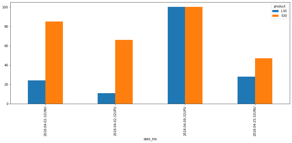
Or as a plot:

[7]:

df_downloaded["product_date"] = df_downloaded["product"] + "-" + df_downloaded["date"]
df_downloaded["date_tile"] = df_downloaded["date"] + "-" + df_downloaded["tile"]
#df_downloaded.pivot(index="product_date", columns="tile", values="cloud_cover").plot.bar(figsize=(16, 6))
df_downloaded.pivot(index="date_tile",
                    columns="product",
                    values="cloud_cover").plot.bar(figsize=(16, 6))

[7]:

<matplotlib.axes._subplots.AxesSubplot at 0x7f5f705a8b80>

../_images/tutorials_Working_with_HLS_datasets_and_nasa_hls_13_1.png

Convert HDF to single-layer GeoTIFFs¶

Note: Starting from nasa_hls version 0.1.1 you can also convert the data to Cloud Optimized GeoTIFFs (COG). This also requires GDAL >= 3.1.

To create COGs use teh option gdal_translate_options="-of COG" in convert_hdf2tiffs.

Single scene¶

[8]:

# L30
nasa_hls.convert_hdf2tiffs(Path("./xxx_uncontrolled_hls/downloads/HLS.L30.T32UNU.2018092.v1.4.hdf"),
                           geotiff_dir,
                           bands=None, # use this to convert only a subset of the bands
                           max_cloud_coverage=100,  # use this to only convert scenes that have lower than specified cloud cover
                          )

[8]:

PosixPath('xxx_uncontrolled_hls/geotiffs/HLS.L30.T32UNU.2018092.v1.4')

[9]:

# S30
nasa_hls.convert_hdf2tiffs(Path("./xxx_uncontrolled_hls/downloads/HLS.S30.T32UNU.2018092.v1.4.hdf"),
                           geotiff_dir,
                           bands=None,
                           max_cloud_coverage=100,
                          )

[9]:

PosixPath('xxx_uncontrolled_hls/geotiffs/HLS.S30.T32UNU.2018092.v1.4')

As a result you get all the (desired) bands in a subfolder of the destination directory. Note the differences between the L30 and S30 files.

[10]:

%%bash
tree xxx_uncontrolled_hls/geotiffs/HLS.L30.T32UNU.2018092.v1.4
tree xxx_uncontrolled_hls/geotiffs/HLS.S30.T32UNU.2018092.v1.4

xxx_uncontrolled_hls/geotiffs/HLS.L30.T32UNU.2018092.v1.4
├── HLS.L30.T32UNU.2018092.v1.4__Blue.tif
├── HLS.L30.T32UNU.2018092.v1.4__Cirrus.tif
├── HLS.L30.T32UNU.2018092.v1.4__Coastal_Aerosol.tif
├── HLS.L30.T32UNU.2018092.v1.4__Green.tif
├── HLS.L30.T32UNU.2018092.v1.4__NIR.tif
├── HLS.L30.T32UNU.2018092.v1.4__QA.tif
├── HLS.L30.T32UNU.2018092.v1.4__Red.tif
├── HLS.L30.T32UNU.2018092.v1.4__SWIR1.tif
├── HLS.L30.T32UNU.2018092.v1.4__SWIR2.tif
├── HLS.L30.T32UNU.2018092.v1.4__TIRS1.tif
└── HLS.L30.T32UNU.2018092.v1.4__TIRS2.tif

0 directories, 11 files
xxx_uncontrolled_hls/geotiffs/HLS.S30.T32UNU.2018092.v1.4
├── HLS.S30.T32UNU.2018092.v1.4__Blue.tif
├── HLS.S30.T32UNU.2018092.v1.4__Cirrus.tif
├── HLS.S30.T32UNU.2018092.v1.4__Coastal_Aerosol.tif
├── HLS.S30.T32UNU.2018092.v1.4__Green.tif
├── HLS.S30.T32UNU.2018092.v1.4__NIR_Broad.tif
├── HLS.S30.T32UNU.2018092.v1.4__NIR_Narrow.tif
├── HLS.S30.T32UNU.2018092.v1.4__QA.tif
├── HLS.S30.T32UNU.2018092.v1.4__Red_Edge1.tif
├── HLS.S30.T32UNU.2018092.v1.4__Red_Edge2.tif
├── HLS.S30.T32UNU.2018092.v1.4__Red_Edge3.tif
├── HLS.S30.T32UNU.2018092.v1.4__Red.tif
├── HLS.S30.T32UNU.2018092.v1.4__SWIR1.tif
├── HLS.S30.T32UNU.2018092.v1.4__SWIR2.tif
└── HLS.S30.T32UNU.2018092.v1.4__Water_Vapor.tif

0 directories, 14 files

Batch of scene¶

[11]:

nasa_hls.convert_hdf2tiffs_batch(df_downloaded[df_downloaded["date"]=="2018-04-02"]["path"].values,
                                 geotiff_dir)

100%|██████████| 4/4 [00:29<00:00,  7.28s/it]

[11]:

[PosixPath('xxx_uncontrolled_hls/geotiffs/HLS.L30.T32UNU.2018092.v1.4'),
 PosixPath('xxx_uncontrolled_hls/geotiffs/HLS.S30.T32UNU.2018092.v1.4'),
 PosixPath('xxx_uncontrolled_hls/geotiffs/HLS.L30.T32UPU.2018092.v1.4'),
 PosixPath('xxx_uncontrolled_hls/geotiffs/HLS.S30.T32UPU.2018092.v1.4')]

Create a clear-sky mask from the QA layer¶

The HLS v1.4 UserGuide helps to understanding and use the QA layer.

We can read in Appendix A. How to decode the bit-packed QA:

Quality Assessment (QA) encoded at the bit level provides concise presentation but is less convenient for users new to this format.

This is really true especially if compare the difficulty in handling the QA layer to handling the fmask or sen2cor SCL layer layer. Because of that and since the masking of invalid pixels / selection of clear sky pixels is so important we will go in a bit more detail here.

The rest of this section shows how to create the default mask and custom masks from the bit encoded AQ layer.

Sample QA layer¶

For illustration purposes we use the QA layer of the HLS.L30.T32UNU.2018092.v1.4 scene.

From the metadata we got the following information about the HDF file:

[12]:

df_downloaded.loc["HLS.L30.T32UNU.2018092.v1.4", ["cloud_cover", "spatial_coverage"]]

[12]:

cloud_cover         24
spatial_coverage    29
Name: HLS.L30.T32UNU.2018092.v1.4, dtype: object

Understand the QA layer¶

The metadata also gives us a QA description. We also find that information in the HLS v1.4 UserGuide:

title

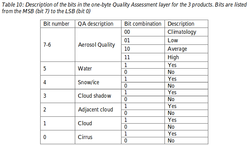
Appendix A of the HLS v1.4 UserGuide shows how to decode the QA bits with simple integer arithmetic. Here we show a way how to do this in Python.

Lets start with the example from the Appendix A:

Suppose we get a decimal QA value 100, which translates into binary 01100100, indicating that the aerosol level is low (bits 6-7), it is water (bit 5), and adjacent to cloud (bit 2).

Derive clear-sky mask from the QA layer¶

The guide gives some advice on how to use the QA layer:

Users are advised to mask out Cirrus, Cloud and Adjacent cloud pixels.

We want to find out here, which rules have been used to calculate the cloud cover we find in in the metadata. There is no explicit information about the used rules.

Therefore we first create a dataframe where the information of the table above is expanded for easier accessability. The dataframe can be created with get_qa_look_up_table.

It contains the QA value (i.e. the integer in the raster), the binary string and a boolean column which indicates if for a given QA value a given QA case (i.e. a row in the table above) is met.

[13]:

lut_qa = nasa_hls.get_qa_look_up_table()
display(lut_qa.head())
display(lut_qa.tail())

	qa_value	binary_string	a_clima	a_low	a_avg	a_high	water	snow	cloud_shadow	adj_cloud	cloud	cirrus	no_water	no_snow	no_cloud_shadow	no_adj_cloud	no_cloud	no_cirrus
0	0	00000000	True	False	False	False	False	False	False	False	False	False	True	True	True	True	True	True
1	1	00000001	True	False	False	False	False	False	False	False	False	True	True	True	True	True	True	False
2	2	00000010	True	False	False	False	False	False	False	False	True	False	True	True	True	True	False	True
3	3	00000011	True	False	False	False	False	False	False	False	True	True	True	True	True	True	False	False
4	4	00000100	True	False	False	False	False	False	False	True	False	False	True	True	True	False	True	True

	qa_value	binary_string	a_clima	a_low	a_avg	a_high	water	snow	cloud_shadow	adj_cloud	cloud	cirrus	no_water	no_snow	no_cloud_shadow	no_adj_cloud	no_cloud	no_cirrus
251	251	11111011	False	False	False	True	True	True	True	False	True	True	False	False	False	True	False	False
252	252	11111100	False	False	False	True	True	True	True	True	False	False	False	False	False	False	True	True
253	253	11111101	False	False	False	True	True	True	True	True	False	True	False	False	False	False	True	False
254	254	11111110	False	False	False	True	True	True	True	True	True	False	False	False	False	False	False	True
255	255	11111111	False	False	False	True	True	True	True	True	True	True	False	False	False	False	False	False

Based on that dataframe it is easy to get the QA integer values for creating a specific mask from it.

Find masking rules resulting in metadata cloud cover¶

As an example let us see if we can calculate the cloud cover from the QA layer by finding the right QA attributes to be masked.

Let’s get the QA values of the sample scene.

[14]:

qa_path = './xxx_uncontrolled_hls/geotiffs/HLS.L30.T32UNU.2018092.v1.4/HLS.L30.T32UNU.2018092.v1.4__QA.tif'
with rasterio.open(qa_path) as qa:
    meta = qa.meta
    qa_array = qa.read()

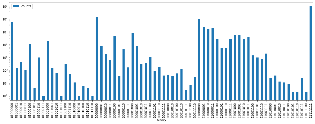
Let’s first visualize the distribution of the values:

[15]:

qa_counts = pd.DataFrame(np.unique(qa_array), columns=["integer"])
qa_counts["binary"] = qa_counts.integer.apply(lambda i: "{0:08b}".format(i))
qa_counts["counts"] = qa_counts.integer.apply(lambda i: (qa_array == i).sum())

n_pix = qa_counts["counts"].sum()
n_obs = qa_counts[qa_counts["integer"] != 255].counts.sum()
print("number of observations (not 255) :", n_obs)
qa_counts.plot.bar(x="binary", y="counts", logy=True, figsize=(18, 6))

number of observations (not 255) : 3930335

[15]:

<matplotlib.axes._subplots.AxesSubplot at 0x7f5f7029ee50>

../_images/tutorials_Working_with_HLS_datasets_and_nasa_hls_30_2.png

Let’s also calculate the percentage of pixels with respect to all pixels and with respect to the observed pixels (i.e. not 255):

[16]:

qa_counts["percent"] = ((qa_counts["counts"] / n_pix) * 100).round(2)
qa_counts["percent_obs"] = ((qa_counts["counts"] / n_obs) * 100).round(2)
qa_counts.loc[qa_counts["integer"] == 255, "percent_obs"] = -0.01
qa_counts.tail()

qa_counts_top_22 = qa_counts.sort_values("percent_obs", ascending=False).head(22)
qa_counts_top_22

[16]:

	integer	binary	counts	percent	percent_obs
19	128	10000000	1389745	10.37	35.36
42	192	11000000	991982	7.41	25.24
0	64	01000000	535713	4.00	13.63
43	193	11000001	228818	1.71	5.82
45	195	11000011	185779	1.39	4.73
44	194	11000010	170090	1.27	4.33
27	136	10001000	79370	0.59	2.02
50	200	11001000	57441	0.43	1.46
51	201	11001001	53104	0.40	1.35
23	132	10000100	44661	0.33	1.14
53	203	11001011	38433	0.29	0.98
49	199	11000111	28472	0.21	0.72
52	202	11001010	28155	0.21	0.72
46	196	11000100	26763	0.20	0.68
8	72	01001000	18869	0.14	0.48
4	68	01000100	10947	0.08	0.28
28	137	10001001	7772	0.06	0.20
20	129	10000001	7303	0.05	0.19
47	197	11000101	5277	0.04	0.13
48	198	11000110	5087	0.04	0.13
25	134	10000110	4114	0.03	0.10
57	207	11001111	1991	0.01	0.05

[17]:

df_downloaded.loc["HLS.L30.T32UNU.2018092.v1.4", ["cloud_cover", "spatial_coverage"]]

[17]:

cloud_cover         24
spatial_coverage    29
Name: HLS.L30.T32UNU.2018092.v1.4, dtype: object

Spatial coverage

[18]:

print("spatial coverage from QA: ", 100 - qa_counts.loc[qa_counts["integer"] == 255, "percent"].values[0])

spatial coverage from QA:  29.340000000000003

Cloud cover

I could not find in the docs how the AQ layer was used to calculate the cloud cover.

With the percentages in qa_counts and the lut_qa dataframe it is now easy to see how different masking decisions influence the percentage of masked pixels for a given QA layer.

The following shows my guesses to find a match for a cloud cover of 24 %.

[19]:

valid = lut_qa.loc[
        ~((lut_qa.cirrus) | (lut_qa.cloud) | (lut_qa.adj_cloud)), "qa_value"
    ].values
percent_valid = qa_counts.loc[qa_counts.integer.isin(valid), "percent_obs"].sum()
100 - percent_valid

[19]:

21.810000000000002

[20]:

valid = lut_qa.loc[
        ~((lut_qa.cloud) | (lut_qa.adj_cloud) | (lut_qa.cloud_shadow)), "qa_value"
    ].values # => 19.8
percent_valid = qa_counts.loc[qa_counts.integer.isin(valid), "percent_obs"].sum()
100 - percent_valid

[20]:

19.75999999999999

[21]:

valid = lut_qa.loc[
        ~((lut_qa.cirrus) | (lut_qa.cloud) | (lut_qa.adj_cloud) | (lut_qa.cloud_shadow)), "qa_value"
    ].values # => 25.8
percent_valid = qa_counts.loc[qa_counts.integer.isin(valid), "percent_obs"].sum()
100 - percent_valid

[21]:

25.769999999999996

[22]:

valid = lut_qa.loc[
        ~((lut_qa.cirrus) | (lut_qa.cloud) | (lut_qa.cloud_shadow)), "qa_value"
    ].values # => 23.7
percent_valid = qa_counts.loc[qa_counts.integer.isin(valid), "percent_obs"].sum()
100 - percent_valid

[22]:

23.67

The winner is: cirrus, cloud and cloud shadow, which somehow makes sense.

That means that we consider the following QA values as clear sky or valid pixels:

[23]:

valid

[23]:

array([  0,   4,  16,  20,  32,  36,  48,  52,  64,  68,  80,  84,  96,
       100, 112, 116, 128, 132, 144, 148, 160, 164, 176, 180, 192, 196,
       208, 212, 224, 228, 240, 244])

Convert the QA layer into a mask¶

Given we know the QA values that we want to consider as valid or invalid pixels we can derive a mask array or GeoTIFF from a GeoTIFF QA layer.

Here we use the function hls_qa_layer_to_mask to quickly test if the masking with the valid values give us the same cloud cover as the mateadata.

Note that you have the following additional options:

keep_255 (bool): If True this keeps the value 255 for the non sensed pixels.
mask_path (str): If a path is given the function will create a raster of the mask there and not output an array.
overwrite (bool): Defines if a file existing at mask_path should be overwritten.

[24]:

for i, row in df_downloaded.iterrows():
    sceneid = Path(row.path).stem
    qa_path = f'xxx_uncontrolled_hls/geotiffs/{sceneid}/{sceneid}__QA.tif'
    if not Path(qa_path).exists():
        continue

    clear_arr = nasa_hls.hls_qa_layer_to_mask(qa_path,
                                              qa_valid=valid,
                                              keep_255=True,
                                              mask_path=None,
                                              overwrite=False)
    n_pix = clear_arr.size
    n_obs = (clear_arr != 255).sum()
    n_cloudy = (clear_arr == 0).sum()
    n_clear = (clear_arr == 1).sum()
    cloud_cover = n_cloudy / (n_clear + n_cloudy)

    print("*" * 90)
    print(qa_path)
    print(f"Number of pixels             : {n_pix}")
    print(f"Number of obs.               : {n_obs}")
    print(f"Number of clear obs.         : {n_clear}")
    print(f"Number of cloudy obs.        : {n_cloudy}")

    print(f"Cloud cover - metadata       : {row.cloud_cover}")
    print(f"Cloud cover - calculated     : {round(cloud_cover * 100, 1) }")

    print(f"Spatial coverage - metadata  : {row.spatial_coverage}")
    print(f"Spatial coverage - calculated: {round((n_obs / n_pix) * 100, 1) }")

******************************************************************************************
xxx_uncontrolled_hls/geotiffs/HLS.L30.T32UNU.2018092.v1.4/HLS.L30.T32UNU.2018092.v1.4__QA.tif
Number of pixels             : 13395600
Number of obs.               : 3930335
Number of clear obs.         : 2999963
Number of cloudy obs.        : 930372
Cloud cover - metadata       : 24.0
Cloud cover - calculated     : 23.7
Spatial coverage - metadata  : 29.0
Spatial coverage - calculated: 29.3
******************************************************************************************
xxx_uncontrolled_hls/geotiffs/HLS.S30.T32UNU.2018092.v1.4/HLS.S30.T32UNU.2018092.v1.4__QA.tif
Number of pixels             : 13395600
Number of obs.               : 13272703
Number of clear obs.         : 1976262
Number of cloudy obs.        : 11296441
Cloud cover - metadata       : 85.0
Cloud cover - calculated     : 85.1
Spatial coverage - metadata  : 100.0
Spatial coverage - calculated: 99.1
******************************************************************************************
xxx_uncontrolled_hls/geotiffs/HLS.L30.T32UPU.2018092.v1.4/HLS.L30.T32UPU.2018092.v1.4__QA.tif
Number of pixels             : 13395600
Number of obs.               : 13395365
Number of clear obs.         : 11980540
Number of cloudy obs.        : 1414825
Cloud cover - metadata       : 11.0
Cloud cover - calculated     : 10.6
Spatial coverage - metadata  : 100.0
Spatial coverage - calculated: 100.0
******************************************************************************************
xxx_uncontrolled_hls/geotiffs/HLS.S30.T32UPU.2018092.v1.4/HLS.S30.T32UPU.2018092.v1.4__QA.tif
Number of pixels             : 13395600
Number of obs.               : 12915488
Number of clear obs.         : 4495212
Number of cloudy obs.        : 8420276
Cloud cover - metadata       : 66.0
Cloud cover - calculated     : 65.2
Spatial coverage - metadata  : 100.0
Spatial coverage - calculated: 96.4

!!! NOTE AND WARNING !!!

There are some small irregularities between the metadata and the calculated values that should be investigated further.

Feel free to do so… (;

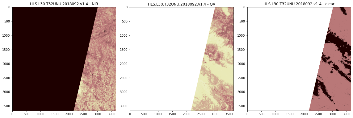
Visualize the mask¶

[25]:

sceneid = "HLS.L30.T32UNU.2018092.v1.4"
src_nir = rasterio.open(f'xxx_uncontrolled_hls/geotiffs/{sceneid}/{sceneid}__NIR.tif')
src_qa = rasterio.open(f'xxx_uncontrolled_hls/geotiffs/{sceneid}/{sceneid}__QA.tif')
qa_path = f'xxx_uncontrolled_hls/geotiffs/{sceneid}/{sceneid}__QA.tif'

clear_arr = nasa_hls.hls_qa_layer_to_mask(qa_path,
                                          qa_valid=valid,
                                          keep_255=True,
                                          mask_path=None,
                                          overwrite=False)

fig, axes = plt.subplots(1, 3, figsize=(16, 8))

axes[0].imshow(src_nir.read(1), vmin=0, vmax=6000, cmap='pink')
axes[0].set_title(sceneid + " - " + "NIR")
axes[1].imshow(src_qa.read(1), vmin=0, vmax=255, cmap='pink')
axes[1].set_title(sceneid + " - " + "QA")
axes[2].imshow(clear_arr, vmin=0, vmax=3, cmap='pink')
axes[2].set_title(sceneid + " - " + "clear")
fig.tight_layout()

../_images/tutorials_Working_with_HLS_datasets_and_nasa_hls_46_0.png