Satellite imagery classification - III
Classification with the help of the Python eobox package.
Introduction
Context and goal
This is the third and last part of a blog post series about using remote sensing data to classify the earth’s surface. In this post we will finally walk through the typical steps it takes to classify remote sensing images with a supervised classifier to derive a land use/land cover map.
We will make use of the remote sensing data from the first part of the series and the OpenStreetMap (OSM) data from the second part of the series.
With these ingredients, a machine learning model can learn patterns between feature vectors and their respective target categories. Then the model can be used to estimate the target category of other feature vectors for creating the land use/land cover map or for model validation by comparing estimated and known target categories. This is the goal of this post.
Processing steps
More specifically, in this post, we will walk through the following steps:
-
Create a reference dataset. Therefore, we need to extract pixel values of the Landsat raster data where it overlays with the polygons of the OSM vector data. Then, we can create a simple two-dimensional table, or reference dataset, which contains, among other information, the labels (land use/land cover information) and features (raster pixel values).
-
Create a training and test dataset. We will do this by splitting the reference dataset.
-
Train a classification model. We will do this with the training set and a random forest classifier.
-
Validate a classification model. We will do this by comparing the known labels of the test dataset with the labels predicted with the trained model.
-
Predict the image data and derive a map. We will do this by predicting all pixels values of the raster, not only the extracted ones.
eobox
For the earth observation specific tasks we will use eobox, a toolbox for processing earth observation data with Python which I started building for learning and practicing purposes. It contains several smaller helpful utilities that might be useful for someone working with remote sensing data in Python. However, I believe that it really might be able to make your life easier if you find yourself in the following situation:
-
You have many large raster files stored as a single-layer GDAL-readable file.
-
The raster files have identical extents, pixel resolution alignment.
-
You want to do pixel-based processing (e.g. over the spectral and/or temporal dimension) and need all pixel values of the whole stack in memory.
-
You want to process the data locally (on your notebook or a server) but the whole stack of the full raster extent does not fit in memory.
-
You do not want to physically split and/or stack the data and you do not want to write boilerplate code to perform chunk-wise processing of the raster stacks.
-
You are patient and okay to wait for more complex processing steps because the package is not optimized for computational performance.
-
The setup and/or learning effort for using another more professional framework is too high and not required for the scope of your problem.
In this post, we are processing a raster dataset that would easily fit in any current standard notebook.
However, the same code works also on raster datasets (such as the 10,000 by 10,000 pixel Sentinel-2 tiles) that are larger than the computer’s memory because internally the computations are done on spatial chunks.
Without the need of writing a lot of boilerplate code, this enables us to run tasks without such as the creation of temporal statistical metrics, virtual time series by linear temporal interpolation (see EOCubeSceneCollection - from level-2 to level-3 products), and the prediction of a sklearn model on large feature stacks.
Additionally, it is easy to write custom functions that can be developed with a spatial chunk of the data and then applied over the whole data EOCubeSceneCollection - custom functions.
However, before using and building on the package, it is important to be aware that it is only a small personal free time project. It is not as mature, performant, supported, stable, and full of features as many professional and/or community-driven framework out there. The following is a non-exhaustive list projects in Python or with a Python API for earth observation data that I find very interesting:
Additionally, you might find more interesting links in the Awesome Geospatial list of geospatial analysis tools.
In this landscape of tools, eobox might be just fine to solve your problem and, compared to some of these frameworks, it might be easier to get started with it. It does not require to set up a database and ingesting or indexing the data (like the Open Data Cube) or to store the data in numpy arrays (like in case of the eo-learn framework). gdalcubes is a very promising project with even more flexibility but it is currently in a very early stage of development and has (so far) only R and not Python bindings. But writing a comprehensive analysis of the scope, strengths, and weaknesses of these projects is a very interesting topic but not the scope of this post – please leave a note in the comments if you are aware of such a comparative analysis. Instead, let us now walk through the steps it takes to classify remote sensing images with a supervised classifier to derive a land use/land cover map.
Supervised classification of remote sensing data
Libraries
We will use the following libraries and modules in this post:
import geopandas as gpd
import matplotlib.pyplot as plt
import numpy as np
import pandas as pd
from pathlib import Path
import rasterio
import seaborn as sns
from shapely.geometry.polygon import Polygon
from shapely.geometry.multipolygon import MultiPolygon
from sklearn.ensemble import RandomForestClassifier
from sklearn.metrics import classification_report, \
                            confusion_matrix
from sklearn.model_selection import train_test_split

from eobox.raster import extract, \
                         load_extracted, \
                         add_vector_data_attributes_to_extracted, \
                         EOCube
from eobox.ml import plot_confusion_matrix, \
                     predict_extended
Create a reference dataset
As described above, a reference dataset is required for supervised classification. A reference dataset contains the target class information, here land use/land cover information from the OSM vector data, and the feature vectors, i.e. the pixel values of the Landsat raster data.
We will use the extract function imported above from the eobox package to perform the extraction:
extract(src_vector: str,
        burn_attribute: str,
        src_raster: list,
        dst_names: list,
        dst_dir: str,
        dist2pb: bool = False,
        dist2rb: bool = False,
        src_raster_template: str = None,
        gdal_dtype: int = 4,
        n_jobs: int = 1) -> int
You can find the latest description of the function and arguments in function’s documentation but we will also work through it in this section.
As we can see from the function signature the function returns an integer, i.e. an exit code of 0 if the process was successful and 1 otherwise.
That means, the function does not directly return the reference dataset but stores the extracted values as NumPy binary files in the directory given via dst_dir.
Later we will load the data with the function load_extracted.
Before we can call the function it is necessary to do some preparatory work for passing the right data to the arguments src_vector, src_raster, and dst_names.
The documentation of src_vector says:
Filename of the vector dataset. Currently, it must have the same CRS as the raster.
And about the related burn_attribute we can read:
Name of the attribute column in the src_vector dataset to be stored with the extracted data. This should usually be a unique ID for the features (points, lines, polygons) in the vector dataset. Note that this attribute should not contain zeros since this value is internally used for pixels that should not be extracted, or, in other words, that do not overlap with the vector data.
Thus, we will create a new dataset from the OSM vector dataset, which is reprojected and has an attribute containing a non-zero polygon ID.
# path of the original OSM vector dataset
path_osm_4326 = "./data_federsee/osm_feedersee_cleansed_4326.geojson"
# path of the new vector dataset that can be passed to
# src_vector
path_osm = "./data_federsee/osm_feedersee_cleansed_32632.geojson"
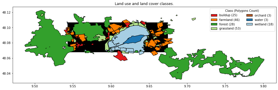
First, we read the file, reproject it the raster CRS and create the non-zero polygon ID and a class ID for the level-1 classes along with colors for the classes, which we will use for plots later.
osm = gpd.read_file(path_osm_4326)
osm = osm.to_crs(epsg=32632) # reproject in the raster CRS
osm["pid"] = range(1, osm.shape[0] + 1) # polygon ids - do not use 0
osm["cid_l1"] = osm["lun_l1"].astype("category").cat.codes + 1

class_lookup_l1 = osm[["lun_l1", "cid_l1"]] \
    .groupby("cid_l1") \
    .first() \
    .reset_index()
class_lookup_l1["color"] = ['#e31a1c',
                            '#ff7f00',
                            '#33a02c',
                            '#b2df8a',
                            '#b15928',
                            '#1f78b4',
                            '#a6cee3']
class_lookup_l1.to_csv("./data_federsee/class_lookup_l1.csv")
class_lookup_l1
| cid_l1 | lun_l1 | color | |
|---|---|---|---|
| 0 | 1 | buildup | #e31a1c |
| 1 | 2 | farmland | #ff7f00 |
| 2 | 3 | forest | #33a02c |
| 3 | 4 | grassland | #b2df8a |
| 4 | 5 | orchard | #b15928 |
| 5 | 6 | water | #1f78b4 |
| 6 | 7 | wetland | #a6cee3 |
In the case here, we also need to convert the geometry type of all polygons to the MultiPolygon type.
osm["geometry"] = [MultiPolygon([geom]) if type(geom) == Polygon \
                   else geom for geom in osm["geometry"]]

assert osm["geometry"].type.unique() == "MultiPolygon"
Else we will get the following error later during extraction.
ValueError:
    Record's geometry type does not match collection schema's geometry type:
        'MultiPolygon' != 'Polygon'
Finally, we can write the new vector dataset to a file.
osm.to_file(path_osm, driver='GeoJSON')
src_raster is the list of file paths of the single-band raster files from which to extract the pixel values.
paths_landsat = Path("./data_federsee/l8_aoi").rglob("**/*.TIF")
paths_landsat = sorted(list(paths_landsat))
And dst_names the list of names corresponding to src_raster. These names will be used for the names of the NumPy binary files and will be the column names when the data is loaded with load_extracted.
Here, the following names contain enough information to be uniquely identifiable.
# dst_names
names_landsat = [f"{fp.stem[17:25]}_{fp.stem[-2::]}" \
                 for fp in  paths_landsat]
Let’s keep all relevant information about the Landsat layers in a DataFrame:
landsat_layers = pd.DataFrame(
    {
        "uname": names_landsat,
        "date": [pd.datetime(int(name[:4]), int(name[4:6]), int(name[6:8])) for name in names_landsat],
        "band": [name.split("_")[1] for name in names_landsat],
        "path": paths_landsat,
    }
)
landsat_layers.to_csv("./data_federsee/landsat_layers.csv")
landsat_layers
| uname | date | band | path | |
|---|---|---|---|---|
| 0 | 20190412_B1 | 2019-04-12 | B1 | data_federsee/l8_aoi/LC08_L1TP_194026_20190412... |
| 1 | 20190412_B2 | 2019-04-12 | B2 | data_federsee/l8_aoi/LC08_L1TP_194026_20190412... |
| 2 | 20190412_B3 | 2019-04-12 | B3 | data_federsee/l8_aoi/LC08_L1TP_194026_20190412... |
| 3 | 20190412_B4 | 2019-04-12 | B4 | data_federsee/l8_aoi/LC08_L1TP_194026_20190412... |
| 4 | 20190412_B5 | 2019-04-12 | B5 | data_federsee/l8_aoi/LC08_L1TP_194026_20190412... |
| 5 | 20190412_B6 | 2019-04-12 | B6 | data_federsee/l8_aoi/LC08_L1TP_194026_20190412... |
| 6 | 20190412_B7 | 2019-04-12 | B7 | data_federsee/l8_aoi/LC08_L1TP_194026_20190412... |
| 7 | 20190818_B1 | 2019-08-18 | B1 | data_federsee/l8_aoi/LC08_L1TP_194026_20190818... |
| 8 | 20190818_B2 | 2019-08-18 | B2 | data_federsee/l8_aoi/LC08_L1TP_194026_20190818... |
| 9 | 20190818_B3 | 2019-08-18 | B3 | data_federsee/l8_aoi/LC08_L1TP_194026_20190818... |
| 10 | 20190818_B4 | 2019-08-18 | B4 | data_federsee/l8_aoi/LC08_L1TP_194026_20190818... |
| 11 | 20190818_B5 | 2019-08-18 | B5 | data_federsee/l8_aoi/LC08_L1TP_194026_20190818... |
| 12 | 20190818_B6 | 2019-08-18 | B6 | data_federsee/l8_aoi/LC08_L1TP_194026_20190818... |
| 13 | 20190818_B7 | 2019-08-18 | B7 | data_federsee/l8_aoi/LC08_L1TP_194026_20190818... |
| 14 | 20190903_B1 | 2019-09-03 | B1 | data_federsee/l8_aoi/LC08_L1TP_194026_20190903... |
| 15 | 20190903_B2 | 2019-09-03 | B2 | data_federsee/l8_aoi/LC08_L1TP_194026_20190903... |
| 16 | 20190903_B3 | 2019-09-03 | B3 | data_federsee/l8_aoi/LC08_L1TP_194026_20190903... |
| 17 | 20190903_B4 | 2019-09-03 | B4 | data_federsee/l8_aoi/LC08_L1TP_194026_20190903... |
| 18 | 20190903_B5 | 2019-09-03 | B5 | data_federsee/l8_aoi/LC08_L1TP_194026_20190903... |
| 19 | 20190903_B6 | 2019-09-03 | B6 | data_federsee/l8_aoi/LC08_L1TP_194026_20190903... |
| 20 | 20190903_B7 | 2019-09-03 | B7 | data_federsee/l8_aoi/LC08_L1TP_194026_20190903... |
The rest of the arguments are quite easy to specify.
We define a destination directory for the extracted data and change arguments dist2pb to True.
For the rest of the arguments, we are fine with the defaults.
The arguments have the following meaning:
dst_dir {str}: Directory to store the data to.
dist2pb {bool}: Create an additional auxiliary layer containing the distance to the closest polygon border for each extracted pixel. Defaults to False.
dist2rb {bool}: Create an additional auxiliary layer containing the distance to the closest raster border for each extracted pixels. Defaults to False.
src_raster_template {str}: A template raster to be used for rasterizing the vectorfile. Usually the first element of src_raster. (default: {None})
gdal_dtype {int}: Numeric GDAL data type, defaults to 4 which is UInt32. See https://github.com/mapbox/rasterio/blob/master/rasterio/dtypes.py for useful look-up tables.
n_jobs {int}: Number of parallel processors to be used for extraction. -1 uses all processors. Defaults to 1.
Now we can perform the extraction.
dir_refset = "./data_federsee/refset"

extract(
    src_vector = path_osm,
    burn_attribute = "pid",
    src_raster = landsat_layers["path"],
    dst_names = landsat_layers["uname"],
    dst_dir = dir_refset,
    dist2pb=True,
    dist2rb=False,
    src_raster_template = None,
    gdal_dtype = 4,
    n_jobs = 1
)
100%|██████████| 176/176 [00:00<00:00, 34128.41it/s]
100%|██████████| 21/21 [00:00<00:00, 863.53it/s]


0
As a result, the following files are created in the destination directory.
list(Path(dir_refset).glob("*"))
[PosixPath('data_federsee/refset/20190903_B6.npy'),
 PosixPath('data_federsee/refset/20190412_B4.npy'),
 PosixPath('data_federsee/refset/aux_coord_x.npy'),
 PosixPath('data_federsee/refset/20190412_B7.npy'),
 PosixPath('data_federsee/refset/20190412_B2.npy'),
 PosixPath('data_federsee/refset/20190412_B3.npy'),
 PosixPath('data_federsee/refset/20190903_B7.npy'),
 PosixPath('data_federsee/refset/20190818_B4.npy'),
 PosixPath('data_federsee/refset/20190818_B7.npy'),
 PosixPath('data_federsee/refset/20190903_B2.npy'),
 PosixPath('data_federsee/refset/burn_attribute_rasterized_pid.tif'),
 PosixPath('data_federsee/refset/20190412_B5.npy'),
 PosixPath('data_federsee/refset/20190903_B4.npy'),
 PosixPath('data_federsee/refset/aux_vector_dist2pb.npy'),
 PosixPath('data_federsee/refset/20190818_B3.npy'),
 PosixPath('data_federsee/refset/20190412_B6.npy'),
 PosixPath('data_federsee/refset/20190818_B2.npy'),
 PosixPath('data_federsee/refset/20190903_B5.npy'),
 PosixPath('data_federsee/refset/20190818_B5.npy'),
 PosixPath('data_federsee/refset/aux_coord_y.npy'),
 PosixPath('data_federsee/refset/20190412_B1.npy'),
 PosixPath('data_federsee/refset/20190903_B3.npy'),
 PosixPath('data_federsee/refset/aux_vector_dist2pb.tif'),
 PosixPath('data_federsee/refset/20190903_B1.npy'),
 PosixPath('data_federsee/refset/20190818_B6.npy'),
 PosixPath('data_federsee/refset/20190818_B1.npy'),
 PosixPath('data_federsee/refset/aux_vector_pid.npy')]
As we can see we get one NumPy binary file per raster layer and additional auxiliary information: the coordinates of the pixels (aux_coord_x, aux_coord_y), the distance to the polygon border (aux_vector_dist2pb) and the polygon ID (aux_vector_pid).
The GeoTIFFs are intermediate data holding the respective information as a raster.
Still, for building and evaluating the classification model we need the target class information along with the pixel values. Additionally, sometimes we have other information stored in the vector data that we need for the analysis. We could later join the data in by using the polygon ID, however, for fast and easy access, we can also store that data as NumPy binary files along with the others. As you can see from the function’s feedback so far only numeric columns are supported.
add_vector_data_attributes_to_extracted(
    ref_vector=path_osm,
    pid='pid',
    dir_extracted=dir_refset,
    overwrite=False)
Skipping column landuse - datatype 'object' not (yet) supported.
Skipping column leaf_type - datatype 'object' not (yet) supported.
Skipping column natural - datatype 'object' not (yet) supported.
Skipping column water - datatype 'object' not (yet) supported.
Skipping column wetland - datatype 'object' not (yet) supported.
Skipping column lun - datatype 'object' not (yet) supported.
Skipping column lun_l1 - datatype 'object' not (yet) supported.
Skipping column color - datatype 'object' not (yet) supported.
Note that all the data derived from the vector data are prefixed with *aux_vector_*. This is true for the polygon ID and distance to the polygon border as well as for the additional attributes derived by add_vector_data_attributes_to_extracted.
list(Path(dir_refset).glob("aux_vector_*.npy"))
[PosixPath('data_federsee/refset/aux_vector_cid_l1.npy'),
 PosixPath('data_federsee/refset/aux_vector_area_m2.npy'),
 PosixPath('data_federsee/refset/aux_vector_dist2pb.npy'),
 PosixPath('data_federsee/refset/aux_vector_pid.npy')]
Now we can use load_extracted to load the data into a pandas DataFrame.
You can load the data you want by an appropriate file pattern or list of file patterns.
Here we use to files patterns that will load all data but makes sure that the auxiliary data is stored in the first columns of the DataFrame.
refset = load_extracted(src_dir=dir_refset,
                        patterns=['aux_*.npy', '2019*.npy'],
                        sort=True)
refset.head()
| aux_coord_x | aux_coord_y | aux_vector_area_m2 | aux_vector_cid_l1 | aux_vector_dist2pb | aux_vector_pid | 20190412_B1 | 20190412_B2 | 20190412_B3 | 20190412_B4 | ... | 20190818_B5 | 20190818_B6 | 20190818_B7 | 20190903_B1 | 20190903_B2 | 20190903_B3 | 20190903_B4 | 20190903_B5 | 20190903_B6 | 20190903_B7 | |
|---|---|---|---|---|---|---|---|---|---|---|---|---|---|---|---|---|---|---|---|---|---|
| 0 | 541470.0 | 5328390.0 | 6.111917e+06 | 3 | 1.000000 | 4 | 9849 | 8872 | 7829 | 7127 | ... | 16736 | 8350 | 6183 | 8866 | 7960 | 7155 | 6278 | 15606 | 7966 | 6091 |
| 1 | 541500.0 | 5328390.0 | 6.111917e+06 | 3 | 1.414214 | 4 | 9806 | 8809 | 7778 | 6967 | ... | 16108 | 8155 | 6099 | 8864 | 7947 | 7123 | 6273 | 14787 | 7619 | 5946 |
| 2 | 541530.0 | 5328390.0 | 6.111917e+06 | 3 | 2.236068 | 4 | 9767 | 8787 | 7724 | 6905 | ... | 14122 | 7252 | 5805 | 8841 | 7929 | 7056 | 6227 | 13124 | 6924 | 5708 |
| 3 | 541560.0 | 5328390.0 | 6.111917e+06 | 3 | 3.162278 | 4 | 9750 | 8787 | 7687 | 6872 | ... | 12640 | 7004 | 5752 | 8828 | 7911 | 7011 | 6194 | 11958 | 6632 | 5630 |
| 4 | 541590.0 | 5328390.0 | 6.111917e+06 | 3 | 4.123106 | 4 | 9780 | 8821 | 7725 | 6943 | ... | 13200 | 7258 | 5846 | 8813 | 7899 | 7044 | 6207 | 12235 | 6843 | 5719 |
5 rows × 27 columns
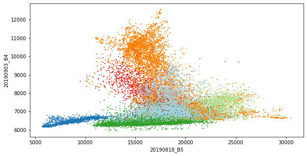
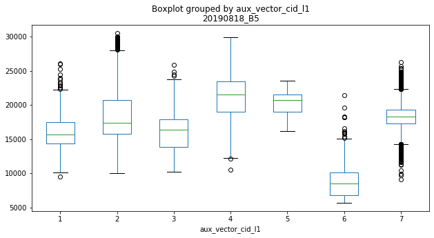
With that data, we can already perform initial explorative data analysis (EDA). For example, we can compare the class distribution of single features (boxplots) or bivariate distributions (scatterplots).
ax = refset.boxplot(by='aux_vector_cid_l1',
                    column=['20190818_B5'],
                    grid=False, figsize=(10, 5))
refset["aux_added_color"] = refset["aux_vector_cid_l1"] \
    .map(class_lookup_l1.set_index("cid_l1")["color"])
ax = refset \
    .plot.scatter(x="20190818_B5", y="20190903_B4",
                  s=1, c=refset["aux_added_color"], figsize=(10, 5))

Of course, there is much more to investigate here but details are not the focus of this post.
Create a training and test dataset
Even though our data is now in a tabular form we should not forget, that we are working with spatial data where spatially close samples are more likely to be similar. This should be considered when a dataset is split into a training and test dataset since they should be relatively independent of each other. Therefore we generate two datasets that are spatially disjointed on polygon level, i.e. we assure that different pixels from the same polygon do not appear in both datasets. Thus, we derive a DataFrame with one sample per polygon and split on polygon-level.
# dataframe with one row per polygon, polygon ID and class ID
aux_polygon = refset[["aux_vector_pid", "aux_vector_cid_l1"]] \
    .groupby("aux_vector_pid") \
    .first() \
    .reset_index()

# polygon IDs of the train and test set
pids_train, pids_test, _, _ = train_test_split(
    aux_polygon[["aux_vector_pid"]],
    aux_polygon["aux_vector_cid_l1"],
    stratify=aux_polygon["aux_vector_cid_l1"],
    test_size=0.5,
    random_state=11)

# pixels belonging to training and test polygons respectively
trainset = refset[
    refset["aux_vector_pid"].isin(pids_train["aux_vector_pid"])]
testset = refset[
    refset["aux_vector_pid"].isin(pids_test["aux_vector_pid"])]

# overview: number of polygons & pixels in training and test set
pd.DataFrame(
    {
        "n_pixels": refset["aux_vector_cid_l1"] \
            .value_counts().sort_index(),
        "n_pixels_train": trainset["aux_vector_cid_l1"] \
            .value_counts().sort_index(),
        "n_pixels_test": testset["aux_vector_cid_l1"] \
            .value_counts().sort_index(),
        "n_polygons": refset \
            .groupby("aux_vector_cid_l1") \
            .apply(lambda x: x["aux_vector_pid"].nunique()),
        "n_polygons_train": trainset \
            .groupby("aux_vector_cid_l1") \
            .apply(lambda x: x["aux_vector_pid"].nunique()),
        "n_polygons_test": testset \
            .groupby("aux_vector_cid_l1") \
            .apply(lambda x: x["aux_vector_pid"].nunique()),
    }
)
| n_pixels | n_pixels_train | n_pixels_test | n_polygons | n_polygons_train | n_polygons_test | |
|---|---|---|---|---|---|---|
| 1 | 1268 | 829 | 439 | 25 | 12 | 13 |
| 2 | 6435 | 2935 | 3500 | 46 | 23 | 23 |
| 3 | 8762 | 7494 | 1268 | 28 | 14 | 14 |
| 4 | 3856 | 1281 | 2575 | 48 | 24 | 24 |
| 5 | 30 | 23 | 7 | 3 | 2 | 1 |
| 6 | 1634 | 11 | 1623 | 3 | 1 | 2 |
| 7 | 10930 | 9808 | 1122 | 18 | 9 | 9 |
We can see that, due to the polygon-based split, we have an extremely unbalanced number of pixels per class and training/test dataset. However, as before, we ignore this detail here and go on with the next step in our walk-through.
Train a classification model
With the training dataset, it is easy to train a simple classification model. We will train a Random Forest classifier here since, compared to other classifiers, it usually performs well even without preprocessing the features (e.g. scaling) or tuning the hyper-parameters.
rf_clf = RandomForestClassifier(n_estimators=200,
                                oob_score=True,
                                n_jobs=-1,
                                random_state=123)
rf_clf = rf_clf.fit(trainset[landsat_layers["uname"]],
                    trainset["aux_vector_cid_l1"])
Validate a classification model
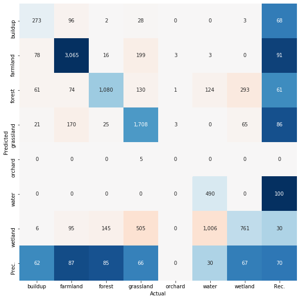
To perform a first validation, or accuracy assessment, of the model we first need to derive the model predictions for the samples of the test dataset. Then we can compare these values with the known target class information. Precision, recall F1-score and the confusion matrix are frequently reported for accuracy assessment. Note that we switch the axes of the confusion matrix since in remote sensing the actual class memberships are more frequently reported in the columns and the predictions in the rows.
y_pred = rf_clf.predict(testset[landsat_layers["uname"]])
y_test = testset["aux_vector_cid_l1"]

print(classification_report(y_test, y_pred))
              precision    recall  f1-score   support

           1       0.68      0.62      0.65       439
           2       0.91      0.88      0.89      3500
           3       0.61      0.85      0.71      1268
           4       0.86      0.66      0.75      2575
           5       0.00      0.00      0.00         7
           6       1.00      0.30      0.46      1623
           7       0.30      0.68      0.42      1122

    accuracy                           0.70     10534
   macro avg       0.62      0.57      0.55     10534
weighted avg       0.80      0.70      0.71     10534
fig, ax = plt.subplots(1, 1, figsize=(10, 10))

cm = confusion_matrix(y_test, y_pred)
ax = plot_confusion_matrix(cm,
                           class_names=class_lookup_l1["lun_l1"],
                           switch_axes=True,
                           ax=ax)
Let’s say we are happy with that result by now. Then we can create a map.
Create a map
The data here is so small, that it would be also quite easy to perform the whole prediction by reading all the data, reshape to a 2-dimensional array or DataFrame, predict, reshape the predictions back to a 3-dimensional raster-like format, and write it to a raster file. But if the data gets larger and does not fit in memory more boilerplate code would be required to perform this process in chunks.
Here we will use the EOCube class from the package eobox.
The EOCube class allows passing any custom function on spatial chunks of single-band raster layers with the same extent and pixel alignment.
It allows us to do the above-mentioned steps in spatial chunks (or windows) and process the data with any custom defined function.
Thus, you can focus on developing the core functionality instead of boilerplate code.
You can also find out more about the class in the tutorials An Intro to EOCube and Visualization with EOCube in the eobox package documentation.
Let us initialize an instance of EOCube with the data we need for prediction.
Therefore, we need a DataFrame defining the layer stack which needs a column named uname with unique names and a column named path with the file paths of the rasters.
We have created such a DataFrame above and can use it here:
landsat_layers.head()
| uname | date | band | path | |
|---|---|---|---|---|
| 0 | 20190412_B1 | 2019-04-12 | B1 | data_federsee/l8_aoi/LC08_L1TP_194026_20190412... |
| 1 | 20190412_B2 | 2019-04-12 | B2 | data_federsee/l8_aoi/LC08_L1TP_194026_20190412... |
| 2 | 20190412_B3 | 2019-04-12 | B3 | data_federsee/l8_aoi/LC08_L1TP_194026_20190412... |
| 3 | 20190412_B4 | 2019-04-12 | B4 | data_federsee/l8_aoi/LC08_L1TP_194026_20190412... |
| 4 | 20190412_B5 | 2019-04-12 | B5 | data_federsee/l8_aoi/LC08_L1TP_194026_20190412... |
eoc = EOCube(landsat_layers, chunksize=2**6)
We want to apply the following core function developed for a DataFrame to the whole raster.
It is an extension of sklearn‘s predict_proba method.
It will return the probabilities, as returned by predict_proba, together with the target class ID (according to the maximum probability) and two confidence layers, the maximum probability and the difference between the maximum and the second-highest probability.
We define the in the next cell, however, the details are not important here. The important message is: You can define any custom function with the following properties:
- The first input argument is a DataFrame where the rows represent pixels and the columns represent single-band raster layers.
- It can have any additional arguments that are needed in the function.
- It returns a DataFrame with the same number of rows, still the pixels, and any number of columns that will later be written to the output raster layers.
# this function can also be imported from eobox as follows:
# from eobox.ml import predict_extended

def predict_extended(df, clf):
    """Derive probabilities, predictions, and condfidence layers.

    Parameters
    ----------
    df : pandas.DataFrame
        DataFrame containing the data matris X to be predicted with
        `clf`.
    clf : sklearn.Classifier
        Trained sklearn classfifier with a `predict_proba` method.

    Returns
    -------
    pandas.DataFrame
        DataFrame with the same number of rows as ``df`` and
        (n_classes + 3) columns.
        The columns contain the class predictions, confidence layers
        (max. probability and the difference between the max.
        and second highest probability), and class probabilities.
    """
    def convert_to_uint8(arr):
        return arr.astype(np.uint8)


    probs = clf.predict_proba(df.values)
    pred_idx = probs.argmax(axis=1)
    pred = np.zeros_like(pred_idx).astype(np.uint8)
    for i in range(probs.shape[1]):
        pred[pred_idx == i] = clf.classes_[i]
    # get reliability layers:
    # maximum probability
    # margin, i.e.maximum probability minus second highest probability
    probs_sorted = np.sort(probs, axis=1)
    max_prob = probs_sorted[:, probs_sorted.shape[1] - 1]
    margin = (
        probs_sorted[:,
                     probs_sorted.shape[1] - 1] \
        - probs_sorted[:,
                       probs_sorted.shape[1] - 2]
    )

    probs = convert_to_uint8(probs * 100)
    max_prob = convert_to_uint8(max_prob * 100)
    margin = convert_to_uint8(margin * 100)

    ndigits = len(str(max(clf.classes_)))
    prob_names = [f"prob_{cid:0{ndigits}d}" for cid in clf.classes_]
    df_result = pd.concat(
        [
            pd.DataFrame({"pred": pred,
                          "max_prob": max_prob,
                          "margin": margin}),
            pd.DataFrame(probs,
                         columns=prob_names),
        ],
        axis=1,
    )
    return df_result
We can apply this function directly on the test set and get the desired outcomes.
pred_ext = predict_extended(testset[landsat_layers["uname"]],
                            rf_clf)
pred_ext.head()
| pred | max_prob | margin | prob_1 | prob_2 | prob_3 | prob_4 | prob_5 | prob_6 | prob_7 | |
|---|---|---|---|---|---|---|---|---|---|---|
| 0 | 3 | 68 | 46 | 0 | 2 | 68 | 7 | 0 | 0 | 21 |
| 1 | 3 | 86 | 74 | 0 | 0 | 86 | 0 | 0 | 0 | 12 |
| 2 | 3 | 91 | 82 | 0 | 0 | 91 | 0 | 0 | 0 | 9 |
| 3 | 3 | 73 | 49 | 0 | 0 | 73 | 2 | 0 | 0 | 24 |
| 4 | 3 | 95 | 91 | 0 | 0 | 95 | 0 | 0 | 0 | 4 |
But how to apply this function, or any other custom function working on the DataFrame representation of a raster stack, on the raster EOCube data?
We can wrap the function in a small function that we then can pass to the apply_and_write method of EOCube.
For development such a function it is useful to get one chunk of data as DataFrame, as it will also happen later in apply_and_write, and see if everything works.
Before we also need some destination file paths for storing the final results. Note that currently the chunks are stored as GeoTiffs and the full image layers as VRTs.
dst_paths = [Path("./data_federsee/map/") \
             / (col + ".vrt") for col in pred_ext]
dst_paths
[PosixPath('data_federsee/map/pred.vrt'),
 PosixPath('data_federsee/map/max_prob.vrt'),
 PosixPath('data_federsee/map/margin.vrt'),
 PosixPath('data_federsee/map/prob_1.vrt'),
 PosixPath('data_federsee/map/prob_2.vrt'),
 PosixPath('data_federsee/map/prob_3.vrt'),
 PosixPath('data_federsee/map/prob_4.vrt'),
 PosixPath('data_federsee/map/prob_5.vrt'),
 PosixPath('data_federsee/map/prob_6.vrt'),
 PosixPath('data_federsee/map/prob_7.vrt')]
ji = 1
eoc_chunk = eoc.get_chunk(ji)

eoc_chunk = eoc_chunk.read_data()
eoc_chunk = eoc_chunk.convert_data_to_dataframe()
eoc_chunk_pred = predict_extended(eoc_chunk.data,
                                  rf_clf).astype("uint8")
eoc_chunk.write_dataframe(result=eoc_chunk_pred,
                          dst_paths=dst_paths)
This produced the following files:
list(Path("./data_federsee/map/").rglob("*.tif"))
[PosixPath('data_federsee/map/xchunks_cs64/prob_4/prob_4_ji-01.tif'),
 PosixPath('data_federsee/map/xchunks_cs64/prob_5/prob_5_ji-01.tif'),
 PosixPath('data_federsee/map/xchunks_cs64/prob_1/prob_1_ji-01.tif'),
 PosixPath('data_federsee/map/xchunks_cs64/pred/pred_ji-01.tif'),
 PosixPath('data_federsee/map/xchunks_cs64/max_prob/max_prob_ji-01.tif'),
 PosixPath('data_federsee/map/xchunks_cs64/prob_2/prob_2_ji-01.tif'),
 PosixPath('data_federsee/map/xchunks_cs64/prob_3/prob_3_ji-01.tif'),
 PosixPath('data_federsee/map/xchunks_cs64/prob_7/prob_7_ji-01.tif'),
 PosixPath('data_federsee/map/xchunks_cs64/margin/margin_ji-01.tif'),
 PosixPath('data_federsee/map/xchunks_cs64/prob_6/prob_6_ji-01.tif')]
Then, if everything works as desired we can wrap these lines in a function as follows and process all chunks with it.
def fun(eoc_chunk, dst_paths, clf):
    eoc_chunk = eoc_chunk.read_data().convert_data_to_dataframe()
    pred = predict_extended(eoc_chunk.data, rf_clf).astype("uint8")
    eoc_chunk.write_dataframe(result=pred, dst_paths=dst_paths)
    return eoc_chunk.ji

eoc.apply_and_write(fun=fun, dst_paths=dst_paths, clf=rf_clf)
  6%|▌         | 1/17 [00:00<00:03,  5.23it/s]

1 chunks already processed and skipped.


100%|██████████| 17/17 [00:03<00:00,  5.13it/s]
As a result, we get all the output layers for the whole image as VRTs:
list(Path("./data_federsee/map/").rglob("*.vrt"))
[PosixPath('data_federsee/map/prob_7.vrt'),
 PosixPath('data_federsee/map/prob_1.vrt'),
 PosixPath('data_federsee/map/pred.vrt'),
 PosixPath('data_federsee/map/prob_3.vrt'),
 PosixPath('data_federsee/map/prob_2.vrt'),
 PosixPath('data_federsee/map/margin.vrt'),
 PosixPath('data_federsee/map/prob_6.vrt'),
 PosixPath('data_federsee/map/max_prob.vrt'),
 PosixPath('data_federsee/map/prob_4.vrt'),
 PosixPath('data_federsee/map/prob_5.vrt')]
These can usually be used as any other raster format.
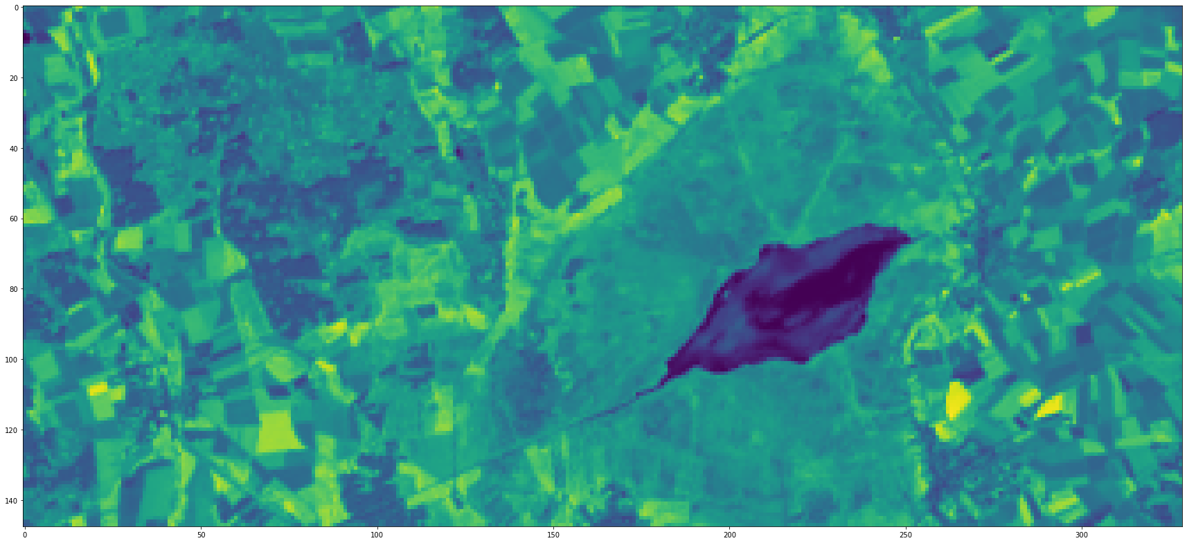
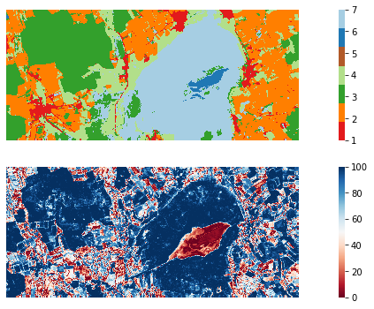
To finalize this section, let us have a look at the prediction and one of the confidence layers.
fig, ax = plt.subplots(2, 1, figsize=(16, 6))

with rasterio.open("./data_federsee/map/pred.vrt") as src:
    arr = src.read()

    sns.heatmap(arr[0,: , :],
                     cmap=sns.color_palette(class_lookup_l1["color"]),
                     square=True,
                     xticklabels=False,
                     yticklabels=False,
                     ax=ax[0],
                    )
with rasterio.open("./data_federsee/map/margin.vrt") as src:
    arr = src.read()
    sns.heatmap(arr[0,: , :],
                     cmap="RdBu",
                     square=True,
                     xticklabels=False,
                     yticklabels=False,
                     ax=ax[1],
                    )
The End
In this post, we walked through the process of classifying remote sensing images. We used the Python package eobox to apply the machine learning capabilities of sklearn to geospatial raster data.
I am happy if this post or the eobox package is helpful for anybody. As always, I am also happy about any critical feedback from which I can learn.