Satellite imagery classification - II
Downloading and preparing OpenStreetMap data
Context and Content
This is the second part of a three parts series about using remote sensing data to classify the earth’s surface. Please read the first part of the series if you are interested in an introduction to the post series and / or in the first part where we downloaded parts of Landsat scenes by leveraging the Cloud Optimized GeoTIFF format.
In this part, after a short introduction to OpenStreetMap (OSM), we will download and prepare land use and land cover data sourced from OSM. The data will be used to create labeled data for the supervised classification task in the next post.
What is OSM?
Let us start with two quotes from the OpenStreetMap Wiki - About OpenStreetMap:
OpenStreetMap is a free, editable map of the whole world that is being built by volunteers largely from scratch and released with an open-content license.
The OpenStreetMap License allows free (or almost free) access to our map images and all of our underlying map data. The project aims to promote new and interesting uses of this data. See “Why OpenStreetMap?" for more details about why we want an open-content map and for the answer to the question we hear most frequently: Why not just use Google maps?
OSM data model
According to the OSM Wiki Features are mappable physical landscape elements. Elements allow us to define where these features are in space and which of and how the elements belong together. Tags tell us more about the elements.
Elements
The OSM database is a collection of the following elements
nodes    : points in space defined by latitude and longitude coordinates
ways     : linear features and area boundaries defined by multiple nodes
relations: sometimes used to explain how other elements work together
Tags
Tags are described in the Wiki as follows:
A tag consists of two items, a key and a value. Tags describe specific features of map elements (nodes, ways, or relations) […]. OpenStreetMap Wiki - Tags
The OpenStreetMap Wiki - Map Features page lists such key value pairs. In this list we can find - among many others - the key natural and landuse. Later we will download the data for our AOI which has been been tagged with one of these two keys. We use the tags’ values as labels for the land use and land cover classification in the next post. Note that also other keys contain useful information for a land use and land cover classification but for this post series we only select two to keep it simple.
Example Federsee
Let us see how the abstract description above looks like in practice.
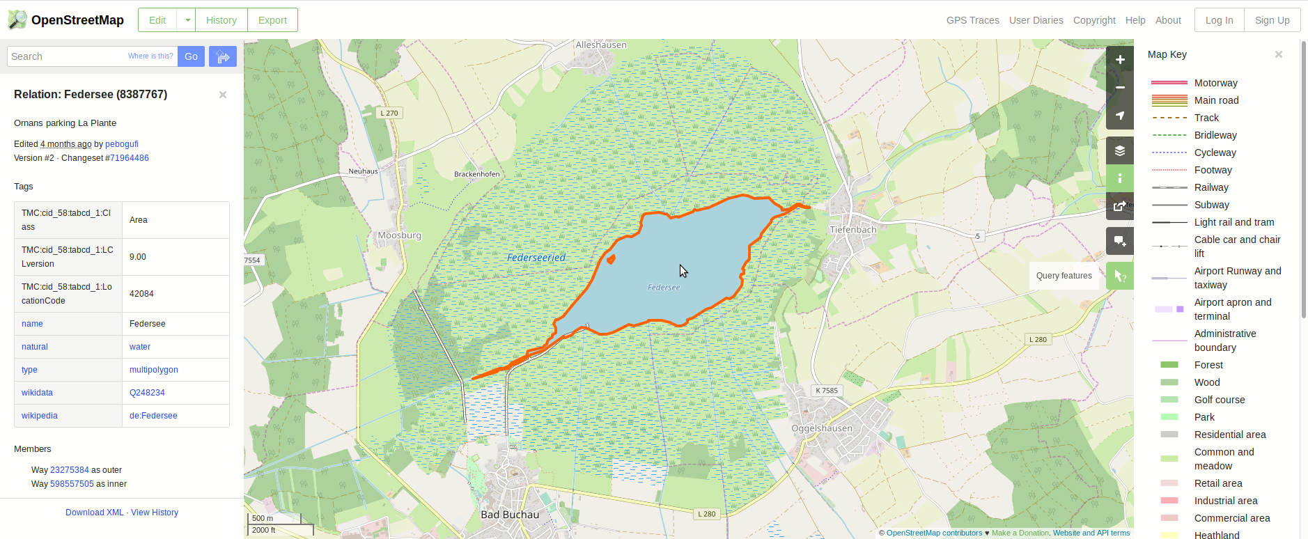
The following screenshot shows OSM representation of the Federsee on www.openstreetmap.org. The Federsee (8387767) is a relation which consists of two ways (see Members), an outer and an inner one since there is an island in the lake. If we click on the IDs of the ways in the lower left corner we would see that each of them is made up by several nodes. These elements allow to draw the feature on the map. Besides that, additional information about the feature is available via the tags, e.g. the name is Federsee, value for the key natural is water, etc. Note that the tags are also used for selecting the style in which to draw a feature.
Download options for OpenStreetMap data
There are several ways how you can get the OSM data. One possibility is to navigate to the AOI in the Export Tab of the OpenStreetMap Webpage. From there you can download the data of an area of interest (AOI) as a OSM XML file.
You can also use the Overpass API which is a read-only API […] optimized for data consumers that need a few elements within a glimpse or up to roughly 10 million elements. A nice post for getting started is Loading Data from OpenStreetMap with Python and the Overpass API which also references Overpass Torbo. The latter is is practical to evaluate queries in the browser. The whole data for the AOI can be queried as follows:
/*
This is a simple map call.
It returns all data in the bounding box.
*/
[out:xml];
(
  node(48.0680, 9.5430, 48.1068, 9.6744);
  <;
);
out meta;
overpy and overpass are two Python APIs for accessing the Overpass API. On October 3rd, 2019 overpy had 110 stars 41 forks and overpass 186 stars, 66 forks.
In this post we use yet another option, i.e. the osmnx package.
This package is very nice because it allows us to download the data of our AOI with a landuse or natural key and convert it in a geopandas.GeoDataFrame in one line of code.
Since we now know better what OSM data is, which part of the data we want to download and which framework we want to use, we can get start with the hands-on part of this post.
Downloading and preparing OSM data with osmnx and pandas
Libraries
Following libraries will be used in this post:
import geopandas as gpd
from matplotlib.patches import Patch
import numpy as np
import osmnx as ox
import pandas as pd
Area of interest
We load the AOI from the GeoJSON ./data_federsee/aoi_federsee_4326.geojson which we stored in the [first part of the series]({% post_url 2019-09-29-1_federsee-blog-series_part-1_cog %}). The content of the file looks as follows:
%%bash

cat ./data_federsee/aoi_federsee_4326.geojson
{
"type": "FeatureCollection",
"crs": { "type": "name", "properties": { "name": "urn:ogc:def:crs:OGC:1.3:CRS84" } },
"features": [
{ "type": "Feature", "properties": { "ID": 1, "Name": "Federsee" }, "geometry": { "type": "Polygon", "coordinates": [ [ [ 9.543, 48.1068 ], [ 9.6744, 48.1068 ], [ 9.6744, 48.068 ], [ 9.543, 48.068 ], [ 9.543, 48.1068 ] ] ] } }
]
}
gdf_aoi_4326 = gpd.read_file(
    "./data_federsee/aoi_federsee_4326.geojson"
)
gdf_aoi_4326
| ID | Name | geometry | |
|---|---|---|---|
| 0 | 1 | Federsee | POLYGON ((9.54300 48.10680, 9.67440 48.10680, ... |
Download OSM data with osmnx
With the osmnx function create_footprints_gdf it does not take more than a line of code to download the data for a specific AOI and footprint type (or OSM tag key) such as ‘building’, ‘landuse’, ‘place’, etc. and convert the data into a geopandas.GeoDataFrame.
Since we are interested in land use and land cover information we download the OSM data of the footprint types ‘natural’ and ‘landuse’.
Download and prepare ‘natural’
Let us download the data and see what we get.
gdf_natural = ox.create_footprints_gdf(
    polygon=gdf_aoi_4326.loc[0, "geometry"],
    footprint_type="natural",
    retain_invalid=True,
)

print(
    "Number of (rows, columns) of the Geodataframe:",
    gdf_natural.shape,
)

print("\nFirst two rows of the GeoDataFrame:")
display(gdf_natural.head(2))

print(
    "\nTransposed description of the GeoDataFrame without geometry, nodes:"
)

# describe() does not work on the three columns we drop here first
gdf_natural.drop(
    ["geometry", "nodes", "members"], axis=1
).describe().transpose()
Number of (rows, columns) of the Geodataframe: (102, 22)

First two rows of the GeoDataFrame:
| nodes | natural | geometry | water | wetland | leaf_cycle | leaf_type | description | intermittent | man_made | ... | operator | species | members | type | TMC:cid_58:tabcd_1:Class | TMC:cid_58:tabcd_1:LCLversion | TMC:cid_58:tabcd_1:LocationCode | name | wikidata | wikipedia | |
|---|---|---|---|---|---|---|---|---|---|---|---|---|---|---|---|---|---|---|---|---|---|
| 31829954 | [356416115, 3959793379, 356416144, 2486677463,... | water | POLYGON ((9.54352 48.10559, 9.54360 48.10561, ... | NaN | NaN | NaN | NaN | NaN | NaN | NaN | ... | NaN | NaN | NaN | NaN | NaN | NaN | NaN | NaN | NaN | NaN |
| 31829956 | [356416148, 2486677471, 2486677470, 356416186,... | water | POLYGON ((9.54280 48.10632, 9.54273 48.10634, ... | NaN | NaN | NaN | NaN | NaN | NaN | NaN | ... | NaN | NaN | NaN | NaN | NaN | NaN | NaN | NaN | NaN | NaN |
2 rows × 22 columns
Transposed description of the GeoDataFrame without geometry, nodes:
| count | unique | top | freq | |
|---|---|---|---|---|
| natural | 102 | 6 | wetland | 27 |
| water | 13 | 2 | pond | 12 |
| wetland | 19 | 4 | wet_meadow | 8 |
| leaf_cycle | 12 | 1 | deciduous | 12 |
| leaf_type | 14 | 1 | broadleaved | 14 |
| description | 1 | 1 | Regenüberlaufbecken | 1 |
| intermittent | 1 | 1 | yes | 1 |
| man_made | 1 | 1 | basin | 1 |
| attraction | 1 | 1 | animal | 1 |
| barrier | 1 | 1 | fence | 1 |
| operator | 1 | 1 | Metallbau Knoll | 1 |
| species | 1 | 1 | chicken, goat, sheep | 1 |
| type | 4 | 1 | multipolygon | 4 |
| TMC:cid_58:tabcd_1:Class | 1 | 1 | Area | 1 |
| TMC:cid_58:tabcd_1:LCLversion | 1 | 1 | 9.00 | 1 |
| TMC:cid_58:tabcd_1:LocationCode | 1 | 1 | 42084 | 1 |
| name | 2 | 2 | Federseeried | 1 |
| wikidata | 1 | 1 | Q248234 | 1 |
| wikipedia | 1 | 1 | de:Federsee | 1 |
We got a GeoDataFrame with 102 rows and 22 columns.
Each row is a feature of the OSM database and is identifiable by the OSM ID stored in the index.
It contains the elements data of OSM in the nodes, geometry and members columns.
Other columns represent the tag keys (column names) and values (values in the cells of the GeoDataFrame).
The column natural is completely filled since we downloaded the footprint type ‘natural’.
All the other tag columns contain various degrees of missing values as can be seen from the described() output.
Remember that our goal is to prepare the data for a land use and land cover classification with 30m resolution imagery (Part 3 of this post series). Therefore it makes sense to only keep ‘Polygon’ and ‘MultiPolygon’ geometries.
rows_keep_natural = gdf_natural.geometry.type.isin(
    ["Polygon", "MultiPolygon"]
)

print("Counts of removed tag values.")
display(
    pd.crosstab(
        gdf_natural.loc[~rows_keep_natural, :].type,
        gdf_natural.loc[~rows_keep_natural, "natural"],
    )
)

gdf_natural = gdf_natural.loc[rows_keep_natural, :]
Counts of removed tag values.
| natural | tree_row |
|---|---|
| row_0 | |
| LineString | 17 |
We also want to keep only the columns / tags which might contain interesting information with regard to classification task.
keep_tag_columns_natural = [
    "natural",
    "water",
    "wetland",
    "leaf_cycle",
    "leaf_type",
]
for col in keep_tag_columns_natural[1::]:
    display(pd.crosstab(gdf_natural["natural"], gdf_natural[col]))
| water | pond | reservoir |
|---|---|---|
| natural | ||
| water | 12 | 1 |
| wetland | marsh | reedbed | swamp | wet_meadow |
|---|---|---|---|---|
| natural | ||||
| wetland | 2 | 6 | 3 | 8 |
| leaf_type | broadleaved |
|---|---|
| natural | |
| wood | 1 |
As we can see leaf_cycle column is empty so we remove it from the initial list. This is probably because there were only values in the removed rows.
# as we can see the leave
keep_tag_columns_natural = [
    "natural",
    "water",
    "wetland",
    "leaf_type",
]

gdf_natural = gdf_natural.loc[
    :, ["geometry"] + keep_tag_columns_natural
]
Download and prepare ‘landuse’
We do the same as above…
gdf_landuse = ox.create_footprints_gdf(
    polygon=gdf_aoi_4326.loc[0, "geometry"],
    footprint_type="landuse",
    retain_invalid=True,
)

rows_keep_landuse = gdf_landuse.geometry.type.isin(
    ["Polygon", "MultiPolygon"]
)
print("Counts of removed tag values.")
display(
    pd.crosstab(
        gdf_landuse.loc[~rows_keep_landuse, :].type,
        gdf_landuse.loc[~rows_keep_landuse, "landuse"],
    )
)
gdf_landuse = gdf_landuse.loc[rows_keep_landuse, :]

print(
    "\nNumber of (rows, columns) of the Geodataframe:",
    gdf_natural.shape,
)

print("\nFirst two rows of the GeoDataFrame:")
display(gdf_landuse.head(2))

print(
    "\nTransposed GeoDataFrame description without geometry, nodes:"
)
# describe() does not work on the three columns we drop here first
gdf_landuse.drop(
    ["geometry", "nodes", "members"], axis=1
).describe().transpose()

keep_tag_columns_landuse = ["landuse", "leaf_type"]
for col in keep_tag_columns_landuse[1::]:
    display(pd.crosstab(gdf_landuse["landuse"], gdf_landuse[col]))

# keep what we need for the classification
gdf_landuse = gdf_landuse.loc[
    :, ["geometry"] + keep_tag_columns_landuse
]
Counts of removed tag values.
Number of (rows, columns) of the Geodataframe: (85, 5)

First two rows of the GeoDataFrame:
| nodes | landuse | geometry | name | toilets:wheelchair | tourism | wheelchair | source | leaf_type | religion | basin | members | type | |
|---|---|---|---|---|---|---|---|---|---|---|---|---|---|
| 8030302 | [60020682, 1369161162, 1369161159, 60020683, 1... | forest | POLYGON ((9.67498 48.09177, 9.67556 48.09173, ... | NaN | NaN | NaN | NaN | NaN | NaN | NaN | NaN | NaN | NaN |
| 8030303 | [60020695, 4878237619, 4878237618, 1369161194,... | forest | POLYGON ((9.67105 48.09603, 9.67099 48.09655, ... | NaN | NaN | NaN | NaN | NaN | NaN | NaN | NaN | NaN | NaN |
Transposed GeoDataFrame description without geometry, nodes:
| leaf_type | broadleaved | mixed | needleleaved |
|---|---|---|---|
| landuse | |||
| forest | 2 | 1 | 2 |
Remove spatial overlaps
Before we combine the data we want to check if there are overlaps between
- the (multi)-polygons of each
GeoDataFrame - between the (multi)-polygons of the two
GeoDataFrames.
For this tutorial we keep it simple and remove these (multi-)polygons as suspicious or ambiguous cases. But of course in a real world scenario it might be worth looking into that cases in more detail to find out if these polygons are useful.
To get overlaps between (multi-)polygons in one Geodataframe we define the following function.
It takes a dataframe and returns None if there are no overlapping polygons and the subset of overlapping polygons otherwise.
def get_overlapping_polygons(gdf):
    """Get the overlap between polygons in the same dataframe."""
    # This is not a performant solution!
    overlaps = []
    for i, row_i in gdf.iterrows():
        for j, row_j in gdf.iterrows():
            if i < j:
                if row_i.geometry.overlaps(row_j.geometry):
                    overlaps.append(i)
                    overlaps.append(j)

    if overlaps:
        return gdf.loc[np.unique(overlaps), :]
    else:
        return None
gdf_natural_overlaps = get_overlapping_polygons(gdf_natural)
gdf_natural_overlaps
There are no overlaping polygons in gdf_natural.
gdf_landuse_overlaps = get_overlapping_polygons(gdf_landuse)
gdf_landuse_overlaps
| geometry | landuse | leaf_type | |
|---|---|---|---|
| 5747104 | POLYGON ((9.57793 48.06533, 9.57764 48.06582, ... | forest | NaN |
| 5747254 | POLYGON ((9.59307 48.06887, 9.59314 48.06881, ... | meadow | NaN |
| 6043203 | POLYGON ((9.72595 48.11495, 9.72592 48.11505, ... | forest | NaN |
| 9945268 | POLYGON ((9.65546 48.09192, 9.65490 48.09161, ... | residential | NaN |
| 601113438 | POLYGON ((9.65429 48.08923, 9.65427 48.08917, ... | farmyard | NaN |
| 601113454 | POLYGON ((9.66902 48.10880, 9.67136 48.10888, ... | farmland | NaN |
There are 6 overlaping polygons in gdf_landuse.
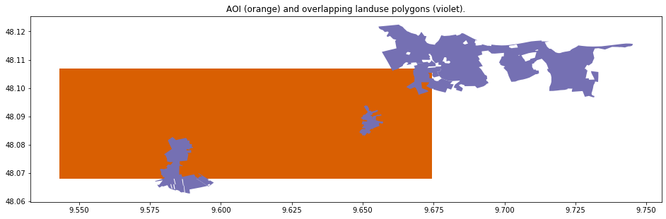
Let us inspect what we loose when we just remove these polygons spatially and in terms of polygon counts per class.
ax = gdf_aoi_4326.plot(color="#d95f02", figsize=(16, 10))
ax = gdf_landuse_overlaps.plot(color="#7570b3", ax=ax)
txt = ax.set_title(
    "AOI (orange) and overlapping landuse polygons (violet)."
)
For the polygon counts comparison we define a function since we will need the same later.
def compare_value_counts(df1, df2, col):
    """Count the values of the same column (col) and create a dataframe with counts and count differences."""
    value_counts_1 = df1[col].value_counts()
    value_counts_2 = df2[col].value_counts()
    df_comparison = pd.concat(
        [
            value_counts_1.rename(f"{col}_1"),
            value_counts_2.rename(f"{col}_2"),
            (value_counts_1 - value_counts_2).rename("1 - 2"),
        ],
        axis=1,
        sort=False,
    )
    return df_comparison


compare_value_counts(
    gdf_landuse,
    gdf_landuse.drop(gdf_landuse_overlaps.index),
    col="landuse",
)
| landuse_1 | landuse_2 | 1 - 2 | |
|---|---|---|---|
| meadow | 71 | 70 | 1 |
| farmland | 48 | 47 | 1 |
| forest | 21 | 19 | 2 |
| farmyard | 14 | 13 | 1 |
| residential | 13 | 12 | 1 |
| orchard | 7 | 7 | 0 |
| allotments | 6 | 6 | 0 |
| commercial | 5 | 5 | 0 |
| plant_nursery | 3 | 3 | 0 |
| industrial | 3 | 3 | 0 |
| cemetery | 2 | 2 | 0 |
| grass | 2 | 2 | 0 |
| basin | 1 | 1 | 0 |
Let us decide that we can get over it when we remove these polygons and do it.
gdf_landuse = gdf_landuse.drop(gdf_landuse_overlaps.index)
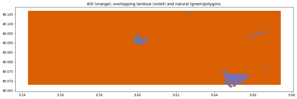
To get overlaping (multi-)polygons between two Geodataframe we can use the overlay functionality of geopandas.
gdf_intersection = gpd.overlay(
    gdf_landuse.reset_index(),
    gdf_natural.reset_index(),
    how="intersection",
)

display(gdf_intersection)

ax = gdf_aoi_4326.plot(color="#d95f02", figsize=(16, 10))
# gdf_intersection.plot(color="#7570b3", ax=ax)
ax = gdf_landuse.loc[gdf_intersection["index_1"]].plot(
    color="#7570b3", ax=ax
)
ax = gdf_natural.loc[gdf_intersection["index_2"]].plot(
    color="#1b9e77", ax=ax
)
txt = ax.set_title(
    "AOI (orange), overlapping landuse (violet) and natural (green)"
    "polygons."
)
| index_1 | landuse | leaf_type_1 | index_2 | natural | water | wetland | leaf_type_2 | geometry | |
|---|---|---|---|---|---|---|---|---|---|
| 0 | 129014138 | commercial | NaN | 216506723 | water | pond | NaN | NaN | POLYGON ((9.64559 48.06889, 9.64563 48.06883, ... |
| 1 | 129014140 | residential | NaN | 600407995 | water | pond | NaN | NaN | POLYGON ((9.64581 48.07079, 9.64586 48.07075, ... |
| 2 | 601767693 | meadow | NaN | 601767688 | grassland | NaN | NaN | NaN | POLYGON ((9.66622 48.07509, 9.66598 48.07507, ... |
| 3 | 715419648 | allotments | NaN | 715419645 | wood | NaN | NaN | NaN | POLYGON ((9.62574 48.10542, 9.62576 48.10541, ... |
| 4 | 715706685 | meadow | NaN | 715706686 | wetland | NaN | NaN | NaN | POLYGON ((9.59961 48.09108, 9.60090 48.09078, ... |
| 5 | 715706685 | meadow | NaN | 715706687 | wetland | NaN | NaN | NaN | POLYGON ((9.59995 48.09326, 9.60021 48.09306, ... |
| 6 | 7283742 | meadow | NaN | 496089851 | scrub | NaN | NaN | NaN | POLYGON ((9.66512 48.09539, 9.66490 48.09536, ... |
compare_value_counts(
    gdf_landuse,
    gdf_landuse.drop(gdf_intersection["index_1"]),
    col="landuse",
)
| landuse_1 | landuse_2 | 1 - 2 | |
|---|---|---|---|
| meadow | 70 | 67 | 3 |
| farmland | 47 | 47 | 0 |
| forest | 19 | 19 | 0 |
| farmyard | 13 | 13 | 0 |
| residential | 12 | 11 | 1 |
| orchard | 7 | 7 | 0 |
| allotments | 6 | 5 | 1 |
| commercial | 5 | 4 | 1 |
| plant_nursery | 3 | 3 | 0 |
| industrial | 3 | 3 | 0 |
| cemetery | 2 | 2 | 0 |
| grass | 2 | 2 | 0 |
| basin | 1 | 1 | 0 |
compare_value_counts(
    gdf_natural,
    gdf_natural.drop(gdf_intersection["index_2"]),
    col="natural",
)
| natural_1 | natural_2 | 1 - 2 | |
|---|---|---|---|
| wetland | 27 | 25 | 2 |
| water | 22 | 20 | 2 |
| wood | 19 | 18 | 1 |
| grassland | 11 | 10 | 1 |
| scrub | 6 | 5 | 1 |
Let us also decide that we can get over that lost.
gdf_landuse = gdf_landuse.drop(gdf_intersection["index_1"])
gdf_natural = gdf_natural.drop(gdf_intersection["index_2"])
Combine ‘landuse’ and ‘natural’
We combine the two GeoDataFrames with a simple non-spatial concatenate operation.
We are confident that we do not get any overlapping polygons since we removed them already.
Still we add an assertion statement here to make sure that this is true.
Also we make the assertion that there we do not have a value for ‘landuse’ and ‘natural’ in any row since we want to combine this information in one column.
gdf_lun = pd.concat([gdf_landuse, gdf_natural], sort=False)

assert get_overlapping_polygons(gdf_lun) is None
assert (gdf_lun[["landuse", "natural"]].isna().sum(axis=1) == 1).all()
Since we did not get an AssertionError our assertions are valid and we can create the label column for the classification task.
Let us call it ‘lun’ for ‘landuse’ and ‘natural’.
gdf_lun["lun"] = gdf_lun["landuse"]
gdf_lun.loc[gdf_lun["landuse"].isna(), "lun"] = gdf_lun["natural"]
Final cleansing
In a final step we
- merge ‘commercial’, ‘industrial’, ‘residential’, ‘farmyard’ into a ‘buildup’ class (knowning that they might include vegetated areas),
- merge ‘meadow’, ‘grassland’ into one ‘grassland’ class,
- merge ‘forest’, ‘wood’ into one ‘forest’ class (knowing that we stretch the meanding of forest here),
- remove polygons of very small size, i.e. smaller than 5 pixels,
- remove label categories with less than 3 polygons (after the steps above).
gdf_lun["lun_l1"] = gdf_lun["lun"]

gdf_lun.loc[
    gdf_lun["lun_l1"].isin(
        ["commercial", "industrial", "residential", "farmyard"]
    ),
    "lun_l1",
] = "buildup"
gdf_lun.loc[
    gdf_lun["lun_l1"].isin(["meadow", "grassland"]), "lun_l1"
] = "grassland"
gdf_lun.loc[
    gdf_lun["lun_l1"].isin(["forest", "wood"]), "lun_l1"
] = "forest"

gdf_lun["area_m2"] = gdf_lun.to_crs(crs={"init": "epsg:32632"}).area
gdf_lun = gdf_lun[gdf_lun["area_m2"] > 5 * 30 * 30]

n_polygons_per_class = gdf_lun["lun_l1"].value_counts()
gdf_lun = gdf_lun[
    gdf_lun["lun_l1"].isin(
        n_polygons_per_class[n_polygons_per_class >= 3].index
    )
]
Visualize and store the cleansed data
Usually we want to use a specific color map for land use / land cover maps.
With geopandas.GeoDataFrame.plot we cannot specify such custom color maps.
Therefore we need create a column containing the colors and create a legend by making use of the lower-level matplotlib plotting functions.
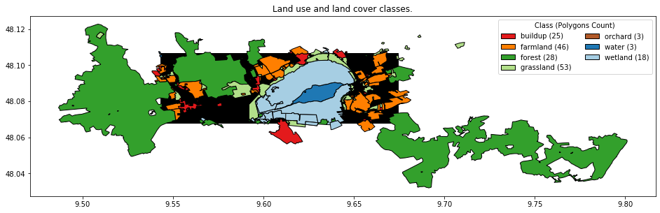
Here is what our labeled data for the classification task in the next post of this series looks like.
# define color code for lun_l1 and add as colors as column
class_color_map = {
    "buildup": "#e31a1c",
    "farmland": "#ff7f00",
    "forest": "#33a02c",
    "grassland": "#b2df8a",
    "orchard": "#b15928",
    "water": "#1f78b4",
    "wetland": "#a6cee3",
}
gdf_lun["color"] = gdf_lun["lun_l1"].map(class_color_map)

# create legend elements
n_polygons_per_class = gdf_lun["lun_l1"].value_counts()
legend_elements = [
    Patch(
        facecolor=value,
        edgecolor="black",
        label=f"{key} ({n_polygons_per_class[key]})",
    )
    for key, value in class_color_map.items()
]


# plot the aoi and the lun_l1 column
ax = gdf_aoi_4326.plot(
    color="black", edgecolor="black", figsize=(16, 10)
)
txt = ax.set_title("Land use and land cover classes.")
ax = gdf_lun.plot(
    color=gdf_lun["color"],
    edgecolor="black",
    ax=ax,
)
# add legend to plot
ax = ax.legend(
    handles=legend_elements,
    title="Class (Polygons Count)",
    loc="upper right",
    ncol=2,
)

Let us store the data such that it is available in the next post.
gdf_lun.to_file(
    "./data_federsee/osm_feedersee_cleansed_4326.geojson",
    driver="GeoJSON",
)
The end
OpenStreetMap is a great open project. The number of people involved and data collected is impressive.
According to the OpenStreetMap stats report run at 2019-10-24 22:00:06 +0000 the numbers look as follows:
Number of users                      5,769,940
Number of uploaded GPS points    7,547,182,003
Number of nodes                  5,549,201,409
Number of ways                     615,216,915
Number of relations                  7,201,811
In this post we downloaded a small part of the OSM data with osmnx and manipulated the data with geopandas and pandas. Together with the satellite data downloaded in the [first part of the series]({% post_url 2019-09-29-1_federsee-blog-series_part-1_cog %}) we do now have the two incredients that we need for creating a land use and land cover map with a supervised classification algorithm in the next and final post of this post series.
Please feel free to leave a comment or contact me if you have any feedback.