Satellite imagery classification - I
Leveraging Cloud Optimized GeoTIFFs to download parts of Landsat scenes
Introduction to the post series
Outline
This is a three parts series about classification of remote sensing images. Remote sensing images are already beautiful enough to only look at, but they can also be used for mapping the earth’s surface. When the task is to map categorical classes, such as forest, water, meadow, farmland, residential area, etc. the task can be solved by classification, often more specifically called land use and/or land cover classification.
In this series we will follow the supervised machine learing paradigm to perform the classification. For that, we need two main ingredients which we will download and prepare in the first two parts of the post series:
In Part 1 of this series we will download the first incredient, i.e. the remote sensing images which will serve as features, or X.
Particularly we will download Landsat scenes and leverage the Cloud Optimized GeoTiff format to only download a subset of the imagery.
In Part 2 we will download and prepare the second ingredient, i.e. georeferenced land use and land cover data which will serve as labels, or y.
Particularly we will use OpenStreetMap data.
In Part 3 we will start cooking and combine the two datasets from the previous parts to train evaluate and apply a model. The model is able to predict the class label given the features, i.e. a list or image pixel values. We will also map the full area of interest (AOI) by applying the model to the full downloaded image.
To solve all these tasks we will use Python.
In Part 3 I will show how the eobox package can be used for the above mentioned tasks to be solved there. I have been working on this package for fun and learning in the end of 2018 but it grew to something that I believe can be helpeful for others.
Let us start with Part 1. But before we dive into it let us import the libraries we need along the way and define the AOI.
Libraries
import folium
import geopandas as gpd
import matplotlib.pyplot as plt
import numpy as np
import pandas as pd
from pathlib import Path
from pyproj import Proj, transform
import rasterio
from shapely import geometry
import subprocess
from tqdm import tqdm
Area of interest
A remote sensing image classification project focuses on a special AOI, i.e. the area in which we want to gain new information or knowledge. Here AOI as around the Feedersee (i.e. feather lake in english) in the heart of Upper Swabia and defined by the bounding box coordinates (as latitudes and longitudes):
north=48.1068
east=9.6744
south=48.0680
west=9.5430
Let us create a geopandas GeoDataFrame from the coordinates and save the AOI as a GeoPackage.
aoi_polygon = geometry.Polygon([[west, north],
                                [east, north],
                                [east, south],
                                [west, south]])

gdf_aoi = gpd.GeoDataFrame(pd.DataFrame(data=[[1, "Federsee"]],
                                        columns=["ID", "Name"]),
                           geometry=[aoi_polygon],
                           crs={'init': 'epsg:4326'})

# safe as GeoPackage
Path("./data_federsee").mkdir(exist_ok=True, parents=True)
gdf_aoi.to_file(filename='./data_federsee/aoi_federsee_4326.geojson', driver='GeoJSON')
Finally let’s see where we are and visualize the AOI with a OSM background layer.
map_osm = folium.Map()
map_osm.fit_bounds([[south, west], [north, east]])
folium.GeoJson(gdf_aoi).add_to(map_osm)
map_osm
Part 1: Leveraging Cloud Optimized GeoTIFFs to download parts of Landsat scenes
Why Cloud Optimized GeoTIFF?
In many, if not most, cases satellite imagery is distributed in quite hugh data packages. This is at least true for the past and present. For example, when you download a Landsat 8 Level-1 GeoTIFF Data Product from USGS EarthExplorer it will have around 900 MB. What if you need only a small part of that imagery such as here where we want to download only a small chunk of some bands of the whole scene? You need to download the whole cake even though you only want a piece or some crumbs of it.
The Cloud Optimized GeoTIFF (COG) format is on the way to chang that. Given that the data provider makes the data available as COGs it allow the clients […] to ask for just the parts of a file they need (quote from Cloud Optimized GeoTIFF).
Data in the Landsat PDS bucket is stored as COGs and this is why we download the data from there.
In Python rasterio is a great package to access to geospatial raster data.
rasterio knows how to handle GOCs since it builds upon GDAL and GDAL handles COGs. Sean Gilles has written a great Jupyter notebook with Advanced features in Rasterio from which I took most of the code below. The notebook demonstrates five advanced features that are useful for developing cloud-native applications. We will make use of those helping us to download only the part of the Landsat imagery covering our AOI.
What to download?
If you are interested in only a few specific Landsat scenes it is convenient to browse and select for the imagery in the EO-Browser of Synergise. A part of the nice search and visualization features it also offers the AWS path of the scenes.
In this post we are interested in the following Landsat scenes:
We want to download the bands 2, 3, 4, 5, 6 and 7 of these scenes but only the parts that overlap with the AOI.
Let us first define variables containing with the scenes and bands we want to download.
scenes = ["LC08_L1TP_194026_20190412_20190412_01_RT",
          "LC08_L1TP_194026_20190818_20190818_01_RT",
          "LC08_L1TP_194026_20190903_20190903_01_RT"
         ]
bands = [f"B{band}" for band in range(1, 8)]
And a function with which we can easily create the paths to the specific file. From the data in the Landsat PDS bucket we know that it is organized by path, row, and scene. So …
def parse_aws_landsat_path(scene, band, ext="TIF"):
    """Parse a scene file path in the aws landsat bucket.
    """
    path = scene.split("_")[2][:3]
    row = scene.split("_")[2][3:]
    path = f"s3://landsat-pds/c1/L8/" \
           f"{path}/{row}/{scene}/{scene}_{band}.{ext}"
    return path

# example
fp = parse_aws_landsat_path("LC08_L1TP_194026_20190818_20190818_01_RT",
                            "B5",
                            "TIF")
fp
's3://landsat-pds/c1/L8/194/026/LC08_L1TP_194026_20190818_20190818_01_RT/LC08_L1TP_194026_20190818_20190818_01_RT_B5.TIF'
We can open this dataset with rasterio as any GDAL readable raster file we would have stored locally.
But before we need to set AWS credentials in our environment.
Even if they are empty. But without we get an CPLE_AWSInvalidCredentialsError.
%env AWS_SECRET_ACCESS_KEY=""
%env AWS_NO_SIGN_REQUEST=""
env: AWS_SECRET_ACCESS_KEY=""
env: AWS_NO_SIGN_REQUEST=""
Now we can get access the data and, for example, get the metadata attribute of it.
with rasterio.open(fp) as src:
    meta = src.meta
meta
{'driver': 'GTiff',
 'dtype': 'uint16',
 'nodata': None,
 'width': 7801,
 'height': 7901,
 'count': 1,
 'crs': CRS.from_epsg(32632),
 'transform': Affine(30.0, 0.0, 462885.0,
        0.0, -30.0, 5531115.0)}
How to download?
How to download with rasterio?
As we have seen the coordinate reference system (CRS) of the Landsat GeoTIFFs is Universal Transverse Mercator (UTM) system.
Our AOI bounding box is given in latitudes and longitudes.
To get the data of the AOI we first need to derive the bounding box coordinates in the CRS of the imagery.
Then we can use these coordinates to create a rasterio.windows.Window instance using the rasterio.windows.from_bounds function.
Finally we are ready to read just the data we need.
Let us converting the AOI to the imagery CRS and taking the bounding box coorinates from there.
gdf_aoi_32632 = gdf_aoi.to_crs({'init': 'epsg:32632'})
gdf_aoi.to_file(filename='data_federsee/aoi_federsee_32632.geojson', driver='GeoJSON')

print(gdf_aoi_32632.bounds.loc[0])

west_32632, south_32632, east_32632, north_32632 = \
    gdf_aoi_32632.bounds.loc[0, :]
minx    5.404216e+05
miny    5.324001e+06
maxx    5.502409e+05
maxy    5.328391e+06
Name: 0, dtype: float64
Note of caution:
This is different from converting the two points and using the coordinates of the resulting points to create the bounding box! This is what I did first, so here is the difference.
proj_4326 = Proj(init='epsg:4326')
proj_32632 = Proj(init='epsg:32632')
west_32632_INEXACT, north_32632_INEXACT = transform(proj_4326,
                                                    proj_32632,
                                                    west, north)
east_32632_INEXACT, south_32632_INEXACT = transform(proj_4326,
                                                    proj_32632,
                                                    east, south)

aoi_polygon_INEXACT = geometry.Polygon([[west_32632_INEXACT, north_32632_INEXACT],
                                        [east_32632_INEXACT, north_32632_INEXACT],
                                        [east_32632_INEXACT, south_32632_INEXACT],
                                        [west_32632_INEXACT, south_32632_INEXACT]])

gdf_aoi_32632.loc[1, :] = (2, "Federsee_INEXACT", aoi_polygon_INEXACT)
map_osm = folium.Map()
map_osm.fit_bounds([[south, west], [south + .01, west + .01]])
folium.GeoJson(gdf_aoi_32632).add_to(map_osm)
map_osm
We can easily show this - see how the lower right and upper left corners are different. So let us delete what we do not need.
del west_32632_INEXACT, north_32632_INEXACT, east_32632_INEXACT, south_32632_INEXACT, aoi_polygon_INEXACT
gdf_aoi_32632 = gdf_aoi_32632.drop(1)
With the correct window we new derive a window aligned with the pixels such that the AOI and that the pixels of the raster subset we derive are exactly aligned with the source raster. If we would not do that, there would be a small shift between the pixel edges.
window = rasterio.windows.from_bounds(west_32632,
                                      south_32632,
                                      east_32632,
                                      north_32632,
                                      transform=meta["transform"]
                                     )
window_aligned = rasterio.windows.Window(col_off=np.floor(window.col_off),
                                         row_off=np.floor(window.row_off),
                                         width=np.ceil(window.width) + 1,
                                         height=np.ceil(window.height) + 1)
# compare
pd.concat([pd.Series(window.todict(), name="window_original"),
           pd.Series(window_aligned.todict(), name="window_aligned")], axis=1)
| window_original | window_aligned | |
|---|---|---|
| col_off | 2584.554036 | 2584.0 |
| row_off | 6757.478236 | 6757.0 |
| width | 327.310592 | 329.0 |
| height | 146.328742 | 148.0 |
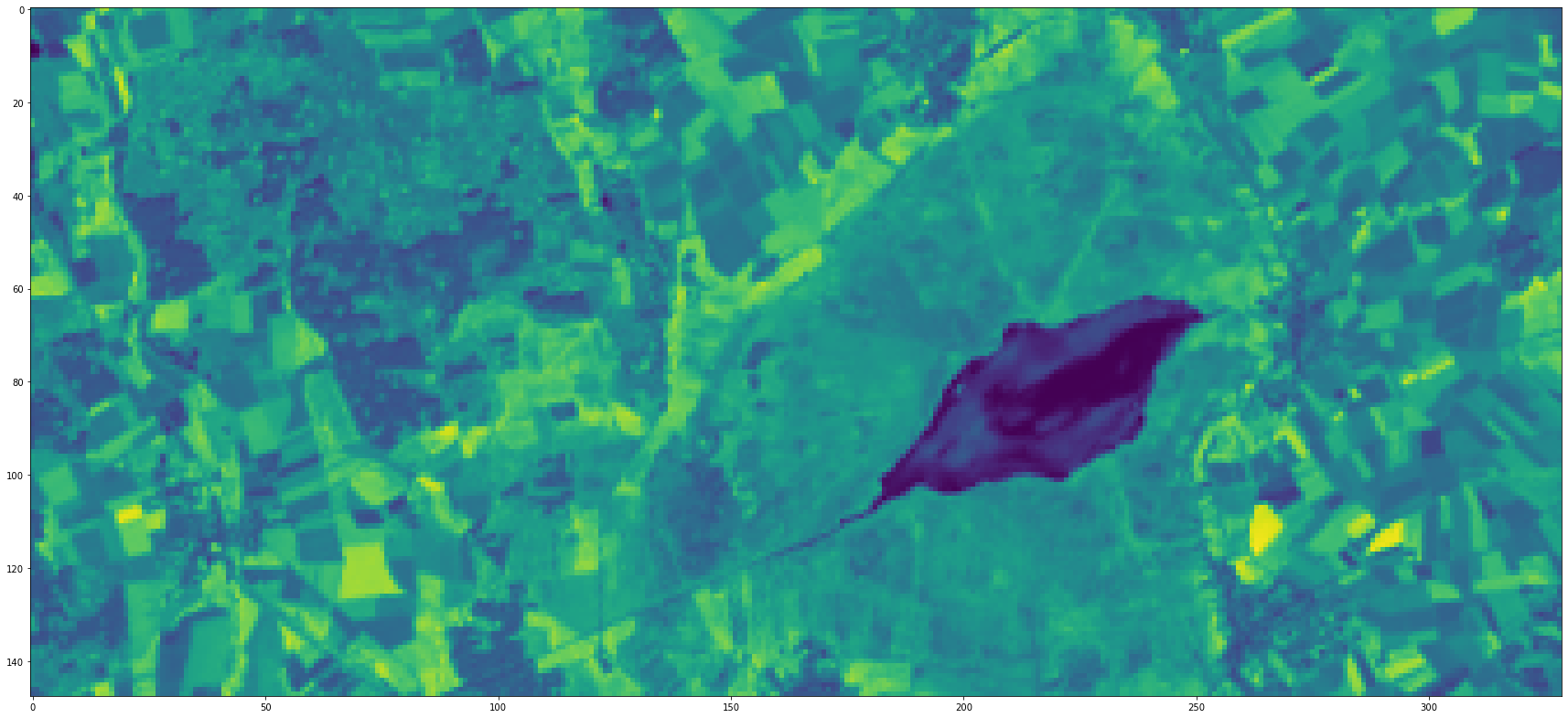
Now we can read the data of our AOI directly in Python.
The code how to safe the data to disc is also there but commented out since we do not want to do this here but with the gdal_translate solution shown below.
# fp_dst = Path("./data_federsee/dev/") / (Path(fp).stem + "_AOI_DEV_rasterio.tif")
# fp_dst.parent.mkdir(exist_ok=True, parents=True)

with rasterio.open(fp) as src:
    arr = src.read(window=window_aligned)

    # kwargs = src.meta.copy()
    # kwargs.update({
    #     'height': window_aligned.height,
    #     'width': window_aligned.width,
    #     'transform': rasterio.windows.transform(window_aligned,
    #                                             src.transform)})

    # with rasterio.open(fp_dst, 'w', **kwargs) as dst:
    #     dst.write(src.read(window=window_aligned))

import seaborn as sns
plt.figure(figsize=(30,15))
plt.imshow(arr[0])
plt.show()

How to download with GDAL?
If it is not necessary to directly load the data in Python it might be easier to use teh comman line tool gdal_translate to store the raster subset locally.
For that we need the following parameters.
gdal_translate
    [-projwin ulx uly lrx lry] [-projwin_srs srs_def]
    src_dataset dst_dataset
Note of caution again:
As above, by using the AOI in the geographic coordinate system we will get an output raster which does not fully cover the AOI. Therefore, we use the AOI in the imagery CRS and expand it for the pixel size of 30 m.
Let us define a function which creates the GDAL command and optionally runs it.
def gdal_translate_landsat_pds_c1_l8(scene: str,
                                     band: str,
                                     gdf_aoi: gpd.GeoDataFrame,
                                     dstdir: Path or str,
                                     process: bool=False,
                                     overwrite: bool=False,
                                     verbose: bool=True):
    """Parse a gdal_translate command to save a subset of a aws landsat 8 pds c1 raster dataset locally."""
    path = scene.split("_")[2][:3]
    row = scene.split("_")[2][3:]
    src_dataset = f"/vsicurl/http://landsat-pds.s3.amazonaws.com/c1/L8/" \
                  f"{path}/{row}/{scene}/{scene}_{band}.TIF"
    dst_dataset = Path(dstdir) / scene / (f"{scene}_{band}.TIF")
    dst_dataset.parent.mkdir(exist_ok=True, parents=True)

    # in case the aoi gdf has more features we use the bounding box embracing all
    projwin = pd.concat([gdf_aoi.bounds[["minx", "miny"]].min(),
                         gdf_aoi.bounds[["maxx", "maxy"]].max()]) \
              .rename({"minx": "ulx",
                       "miny": "lry",
                       "maxx": "lrx",
                       "maxy": "uly"})

    cmd = "gdal_translate " \
          f"-projwin {projwin['ulx']} {projwin['uly']} {projwin['lrx'] + 30} {projwin['lry'] - 30} " \
          f"{str(src_dataset)} " \
          f"{str(dst_dataset)}"
    exit_code = np.nan
    if process:
        if overwrite or not dst_dataset.exists():
            if verbose:
                print("PROCESSING")
            exit_code = subprocess.check_call(cmd, shell=True)
        else:
            if verbose:
                print(f"Processing skipped. File exists: {str(dst_dataset)}")
                print(cmd)
    return cmd, exit_code
An example command looks as follows:
cmd, exit_code = gdal_translate_landsat_pds_c1_l8(scene=scenes[0],
                                                  band="B5",
                                                  gdf_aoi=gdf_aoi_32632,
                                                  dstdir="./data_federsee/dev",
                                                  process=False,
                                                  overwrite=False,
                                                  verbose=True)
cmd
'gdal_translate -projwin 540421.6210704312 5328390.652911871 550270.9388222749 5323970.790656615 /vsicurl/http://landsat-pds.s3.amazonaws.com/c1/L8/194/026/LC08_L1TP_194026_20190412_20190412_01_RT/LC08_L1TP_194026_20190412_20190412_01_RT_B5.TIF data_federsee/dev/LC08_L1TP_194026_20190412_20190412_01_RT/LC08_L1TP_194026_20190412_20190412_01_RT_B5.TIF'
Download
Remember the task - we want to download the bands 2, 3, 4, 5, 6 and 7 of the three scenes above but only the parts that overlap with the AOI.
Now we have everything together such that this task can be solved by a very simple for-loop.
for i, scene in enumerate(scenes):
    print(f"{scene} - {i+1} / {len(scenes)}")
    for band in tqdm(bands, total=len(bands)):
        cmd, exit_code = gdal_translate_landsat_pds_c1_l8(scene=scene,
                                                          band=band,
                                                          gdf_aoi=gdf_aoi_32632,
                                                          dstdir="./data_federsee/l8_aoi",
                                                          process=True,
                                                          overwrite=False,
                                                          verbose=False)
  0%|          | 0/7 [00:00<?, ?it/s]

LC08_L1TP_194026_20190412_20190412_01_RT - 1 / 3


100%|██████████| 7/7 [00:47<00:00,  6.79s/it]
  0%|          | 0/7 [00:00<?, ?it/s]

LC08_L1TP_194026_20190818_20190818_01_RT - 2 / 3


100%|██████████| 7/7 [00:48<00:00,  6.91s/it]
  0%|          | 0/7 [00:00<?, ?it/s]

LC08_L1TP_194026_20190903_20190903_01_RT - 3 / 3


100%|██████████| 7/7 [00:48<00:00,  7.03s/it]
The end
Great, we have downloaded the first ingredient required for the classification task to be solve in the third post of this series. In the next post we will get some georeferenced land use and land cover labels for the same area from OpenStreetMap.
At the same time I have learned some things about Cloud Optimized GeoTIFFs. Particularly that it can save a lot of web traffic if we are only interested in a small part of raster datasets that cover much larger footprints. For example here we ended up downloadint 2MB. If we hat to downloaded the full three Landsat scene that would have summed up to around 3 x 900 MB and quite some more lines of code to get the data subset we wanted.
So in my opinion Cloud Optimized GeoTIFF is really an amazing raster format which we will see and use more and more in the future. In fact, the Collection 2 Level-2 Landsat data will be realeased in COG format by the U.S. Geological Survey (USGS). Which is great.
Feedback
You are more than welcome to leave a comment if you have some thoughts you like to share.
I would love to hear what you liked, what you missed, where you agree or disagree, what you would solve in a different way or any other thoughts.